Lecture 05: GWAS in R

PUBH 8878, Statistical Genetics

Overview

This session walks through a minimal GWAS workflow in R using SNPRelate and GENESIS. There exist many tools for GWAS, including PLINK, BOLT-LMM, REGENIE, SAIGE, and others. Here, we focus on GENESIS to illustrate the key steps.

We work with a small example GDS bundled with GENESIS to keep runtime short while illustrating the full pipeline:

1. Quality control (variant- and sample‑level)
2. LD pruning for structure/relatedness tasks
3. Relatedness (KING‑robust) and population structure (PC‑AiR)
4. Null model fitting (linear mixed model)
5. Single‑variant association and diagnostics (QQ, λGC)

Setup

1library(SNPRelate)
2library(GENESIS)
3library(GWASTools)
4library(qqman)
library(ggplot2)
library(dplyr)
library(readr)
set.seed(8878)

1

SNPRelate (Zheng et al., 2012) for GDS file handling and genotype data management (Zheng et al., 2012)

2

GENESIS for genome-wide association analysis and relatedness estimation (Manichaikul et al., 2010; Conomos et al., 2015)

3

GWASTools for genotype data management and quality control

4

qqman for creating Q-Q and Manhattan plots

Step 1: Accessing and Loading Data

HapMap 3

• HapMap3 is an integrated reference of common and low-frequency alleles. The project genotyped 1.6 million common SNPs in 1,184 reference individuals from 11 global populations. (The International HapMap 3 Consortium, 2010)
• The project mapped linkage disequilibrium (LD) patterns used for tag‑SNP selection and served as an early imputation reference. (The International HapMap 3 Consortium, 2010; The International HapMap Consortium, 2005)
• Here, we will use a small subset from ASW (African ancestry in the Southwest USA) and MXL (Mexican ancestry in Los Angeles) samples

1gdsfile <- system.file("extdata", "HapMap_ASW_MXL_geno.gds", package = "GENESIS")

2g <- SNPRelate::snpgdsOpen(gdsfile)

3samp.id <- read.gdsn(index.gdsn(g, "sample.id"))
snp.id <- read.gdsn(index.gdsn(g, "snp.id"))
chr <- read.gdsn(index.gdsn(g, "snp.chromosome"))
pos <- read.gdsn(index.gdsn(g, "snp.position"))

1

Locate the example GDS file included with the GENESIS package

2

Open the GDS file for random access to genotype data

3

Read sample IDs, SNP IDs, chromosome numbers, and positions from the GDS file

We can also download the associated metadata

metadata <- readr::read_tsv("https://ftp.ncbi.nlm.nih.gov/hapmap/genotypes/hapmap3_r3/relationships_w_pops_041510.txt", show_col_types = FALSE)
head(metadata)

# A tibble: 6 × 7
  FID   IID     dad     mom       sex pheno population
  <chr> <chr>   <chr>   <chr>   <dbl> <dbl> <chr>     
1 2427  NA19919 NA19908 NA19909     1     0 ASW       
2 2431  NA19916 0       0           1     0 ASW       
3 2424  NA19835 0       0           2     0 ASW       
4 2469  NA20282 0       0           2     0 ASW       
5 2368  NA19703 0       0           1     0 ASW       
6 2425  NA19902 NA19900 NA19901     2     0 ASW       

metadata |>
    mutate(population = case_when(population == "MEX" ~ "MXL", 
    TRUE ~ population))

# A tibble: 1,397 × 7
   FID   IID     dad     mom       sex pheno population
   <chr> <chr>   <chr>   <chr>   <dbl> <dbl> <chr>     
 1 2427  NA19919 NA19908 NA19909     1     0 ASW       
 2 2431  NA19916 0       0           1     0 ASW       
 3 2424  NA19835 0       0           2     0 ASW       
 4 2469  NA20282 0       0           2     0 ASW       
 5 2368  NA19703 0       0           1     0 ASW       
 6 2425  NA19902 NA19900 NA19901     2     0 ASW       
 7 2425  NA19901 0       0           2     0 ASW       
 8 2427  NA19908 0       0           1     0 ASW       
 9 2430  NA19914 0       0           2     0 ASW       
10 2470  NA20287 0       0           2     0 ASW       
# ℹ 1,387 more rows

Step 2: Pre-Modeling QC

Genotype quality control

Filtering for minor allele frequency (MAF)

• SNP-chips often determine genotypes based on intensities for each allele
• When MAF is low, genotype clusters can overlap, leading to genotyping errors

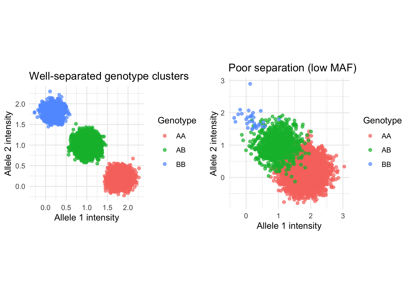
We can compute various statistics regarding allele frequency using snpgdsSNPRateFreq

af <- snpgdsSNPRateFreq(g)
str(af)
maf <- af$MinorFreq

List of 3
 $ AlleleFreq : num [1:20000] 0.39 0.494 0.101 0.486 0.445 ...
 $ MinorFreq  : num [1:20000] 0.39 0.494 0.101 0.486 0.445 ...
 $ MissingRate: num [1:20000] 0 0 0 0 0.00578 ...

We can see that af contains both minor allele frequency and missing rate per SNP.

data.frame(maf = maf) |>
    mutate(maf_le05 = maf < 0.05) |>
    ggplot(aes(x = maf, fill = maf_le05)) +
    geom_histogram(binwidth = 0.01, color = "black") +
    geom_vline(xintercept = c(0.05), linetype = "dashed", color = "red") +
    theme_minimal() +
    viridis::scale_fill_viridis(discrete = TRUE, end = .9, begin = .2) +
    labs(fill = "MAF < .05")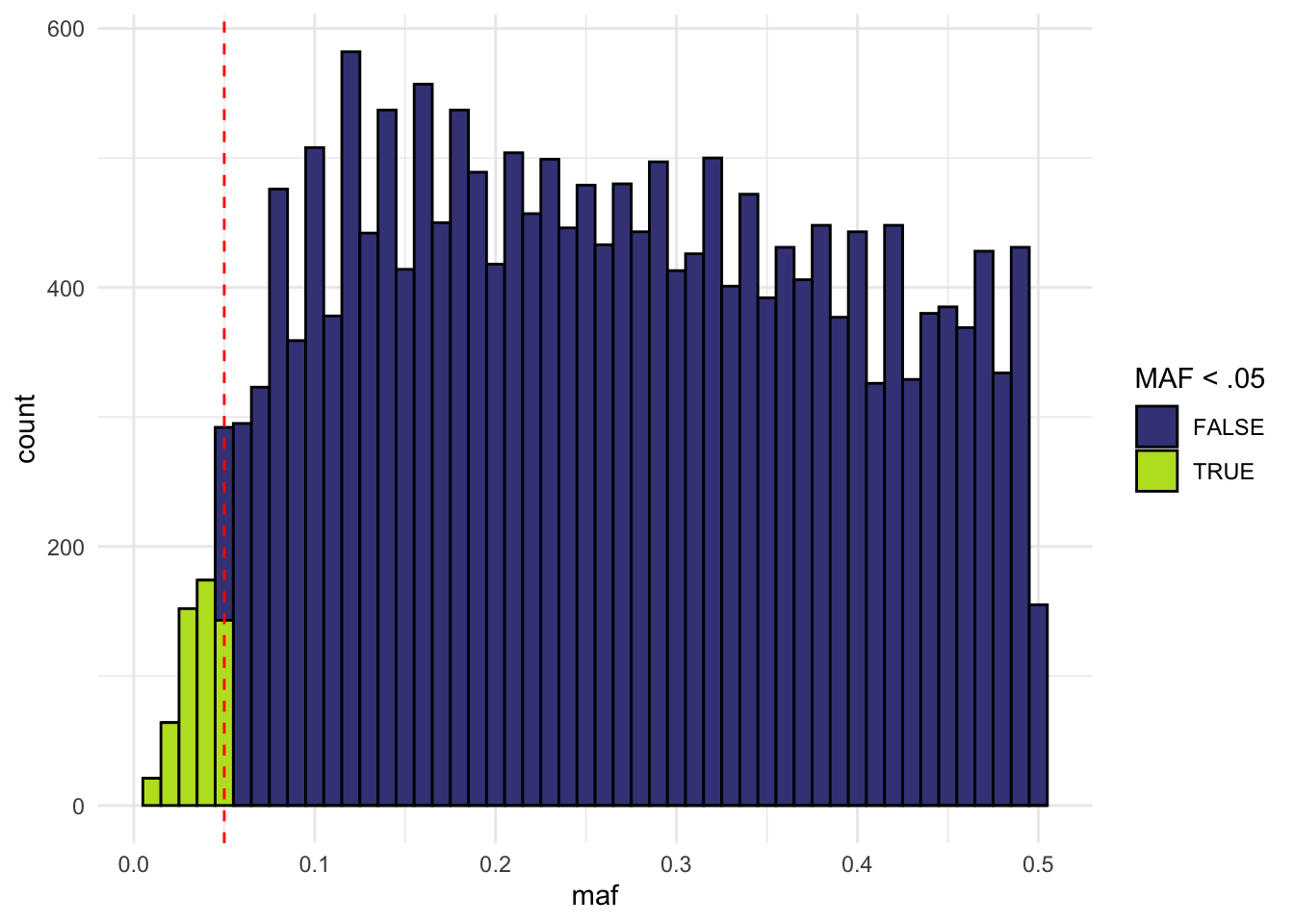

Variant missingness

• Missingness can indicate genotyping errors or batch effects
• Missingness can be non-random with respect to phenotype or ancestry
• Typically filter variants with > 2% missingness
• We can use the missingness results from our af object
• Additionally, we can retrieve the genotype matrix itself, and manually compute the rate per SNP

G <- snpgdsGetGeno(g, with.id = TRUE)

Genotype matrix: 20000 SNPs X 173 samples

geno_mat <- G$genotype
dim(geno_mat)

[1] 20000   173

Indexing in R goes rows-by-columns. So, For geno_mat, the SNPs are rows and the samples are columns. We can inspect subset of the matrix:

geno_mat[10:20, 1:10]

      [,1] [,2] [,3] [,4] [,5] [,6] [,7] [,8] [,9] [,10]
 [1,]    2    0    0    1    0    1    0    1    2     0
 [2,]    0    1    1    1    1    0    0    0    2     0
 [3,]    1    1    1    1    0    0    1    0    2     1
 [4,]    0    0    0    0    0    0    0    0    0     1
 [5,]    0    0    0    0    0    0    0    0    0     0
 [6,]    1    0    1    1    0    0    0    2    1     0
 [7,]    2    1    1    1    0    0    0    2    0     1
 [8,]    0    0    0    0    1    1    0    0    2     0
 [9,]    1    0    0   NA    0    1    0    2    0     0
[10,]    1    1    0    1    1    1    1    0    0     0
[11,]    1    0    1    0    1    1    0    2    1     0

SNPRelate allows for four possible values stored in the genotype matrix: 0, 1, 2, 3. Consider a bi-allelic SNP site with possible alleles A and B.

• 0 indicates BB
• 1 indicates AB
• 2 indicates AA
• 3 indicates a missing genotype

For multi-allelic sites, it is a count of the reference allele.

miss_var_manual <- rowMeans(is.na(geno_mat))
miss_var <- af$MissingRate 
identical(miss_var, miss_var_manual)

[1] TRUE

data.frame(miss_var = miss_var) |>
    mutate(miss_var_gt02 = miss_var > 0.02) |>
    ggplot(aes(x = miss_var, fill = miss_var_gt02)) +
    geom_histogram(binwidth = 0.001, color = "black") +
    geom_vline(xintercept = c(0.02), linetype = "dashed", color = "red") +
    theme_minimal() +
    viridis::scale_fill_viridis(discrete = TRUE, end = .9, begin = .2) +
    labs(fill = "Missing > .02")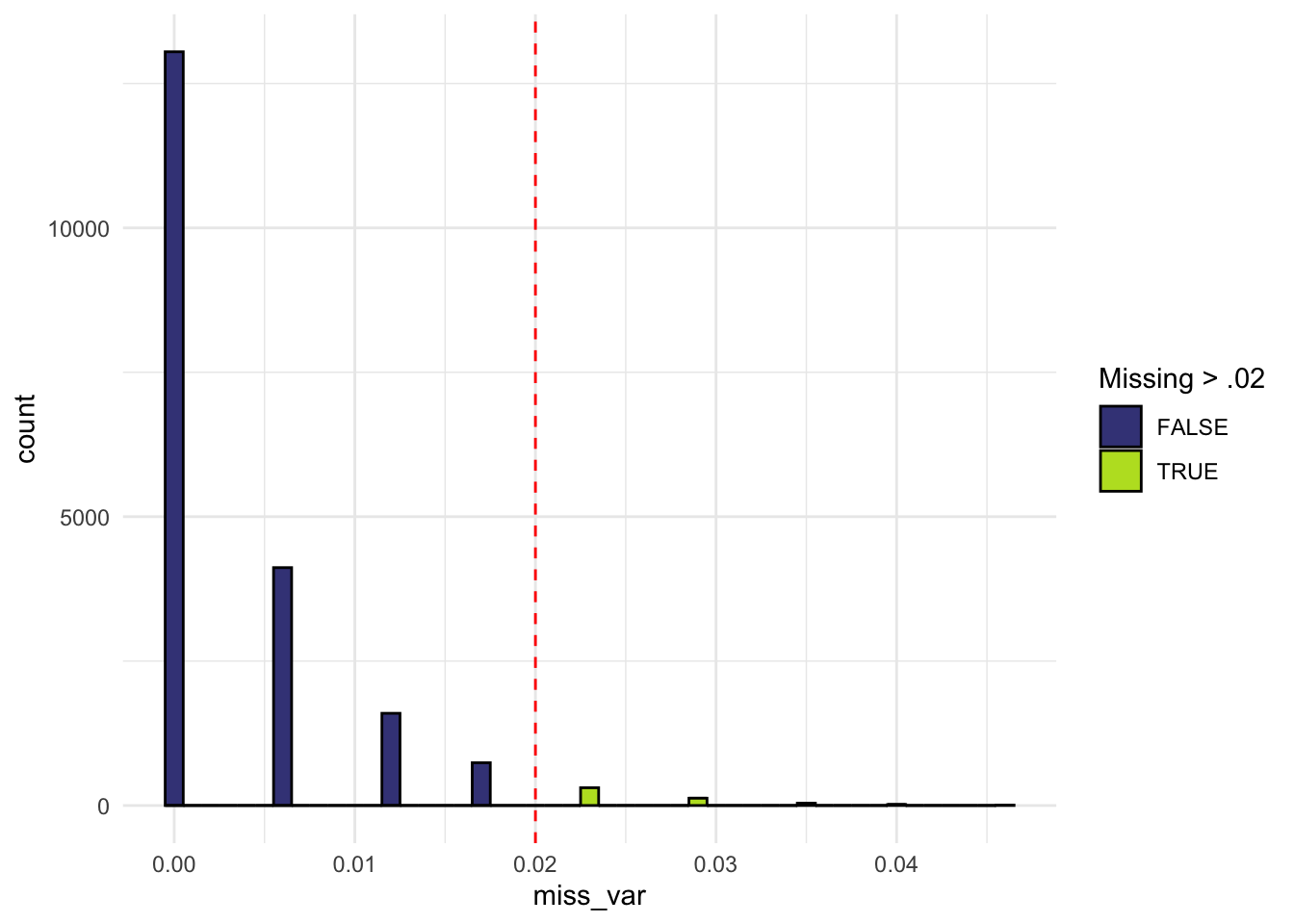

Sample-level missingness & heterozygosity

• Samples with high missingness may have poor DNA quality or technical issues
• Samples with extreme heterozygosity rates may be contaminated or mislabelled

samp_miss <- snpgdsSampMissRate(g)

data.frame(samp_miss = samp_miss) |>
    mutate(samp_outlier = samp_miss > 0.02) |>
    ggplot(aes(x = samp_miss, fill = samp_outlier)) +
    geom_histogram(binwidth = 0.01, color = "black") +
    geom_vline(xintercept = c(0.02), linetype = "dashed", color = "red") +
    theme_minimal() +
    labs(title = "Sample missingness", x = "Missing rate")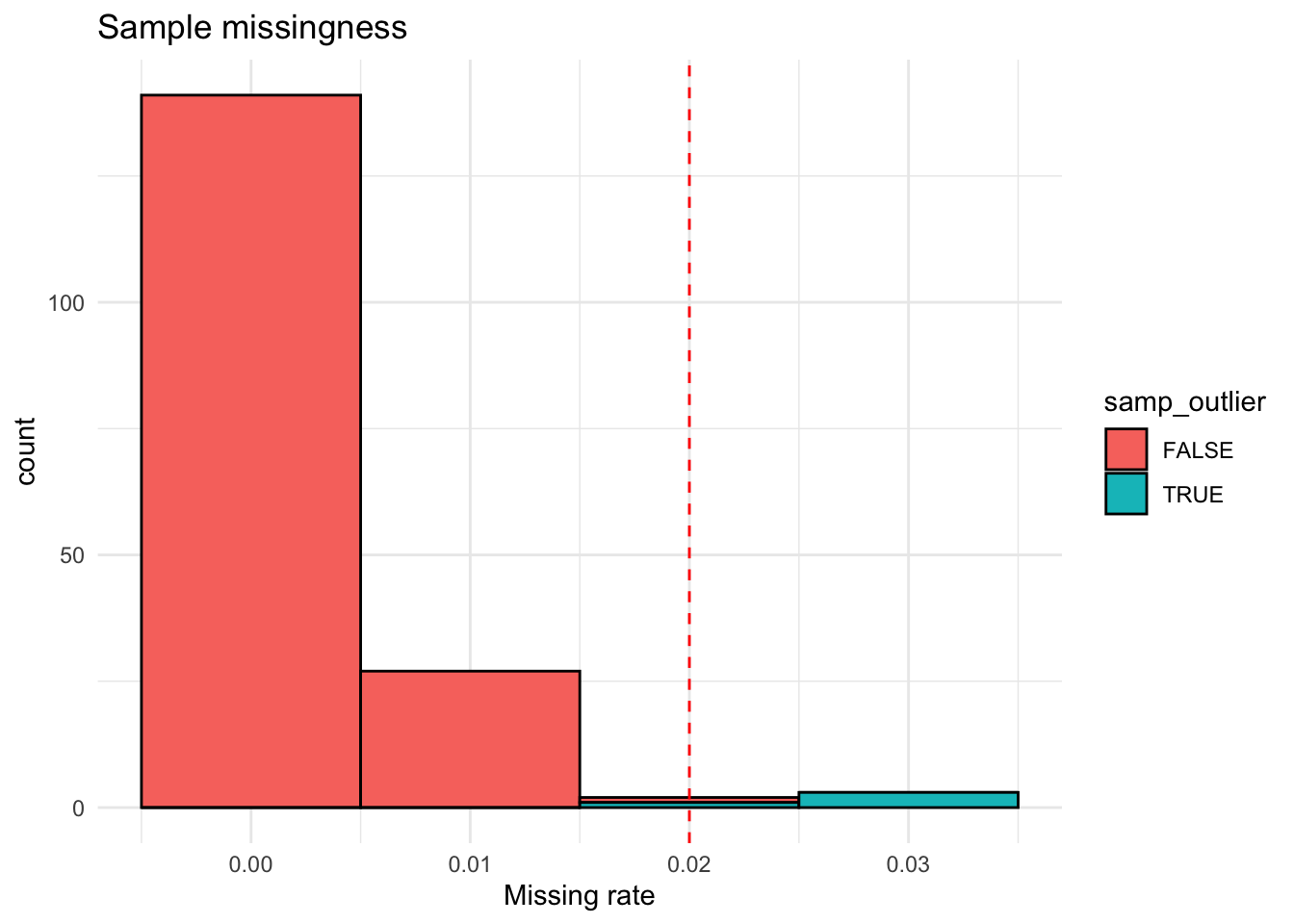

het_rate <- colMeans(geno_mat == 1, na.rm = TRUE)

data.frame(het_rate = het_rate) |>
    mutate(het_outlier = abs(scale(het_rate)) > 3) |>
    ggplot(aes(x = het_rate, fill = het_outlier)) +
    geom_histogram(binwidth = 0.01, color = "black") +
    geom_vline(xintercept = c(mean(het_rate) + 3 * sd(het_rate),
                              mean(het_rate) - 3 * sd(het_rate)),
               linetype = "dashed", color = "red") +
    theme_minimal() +
    labs(title = "Heterozygosity rate", x = "Heterozygosity rate")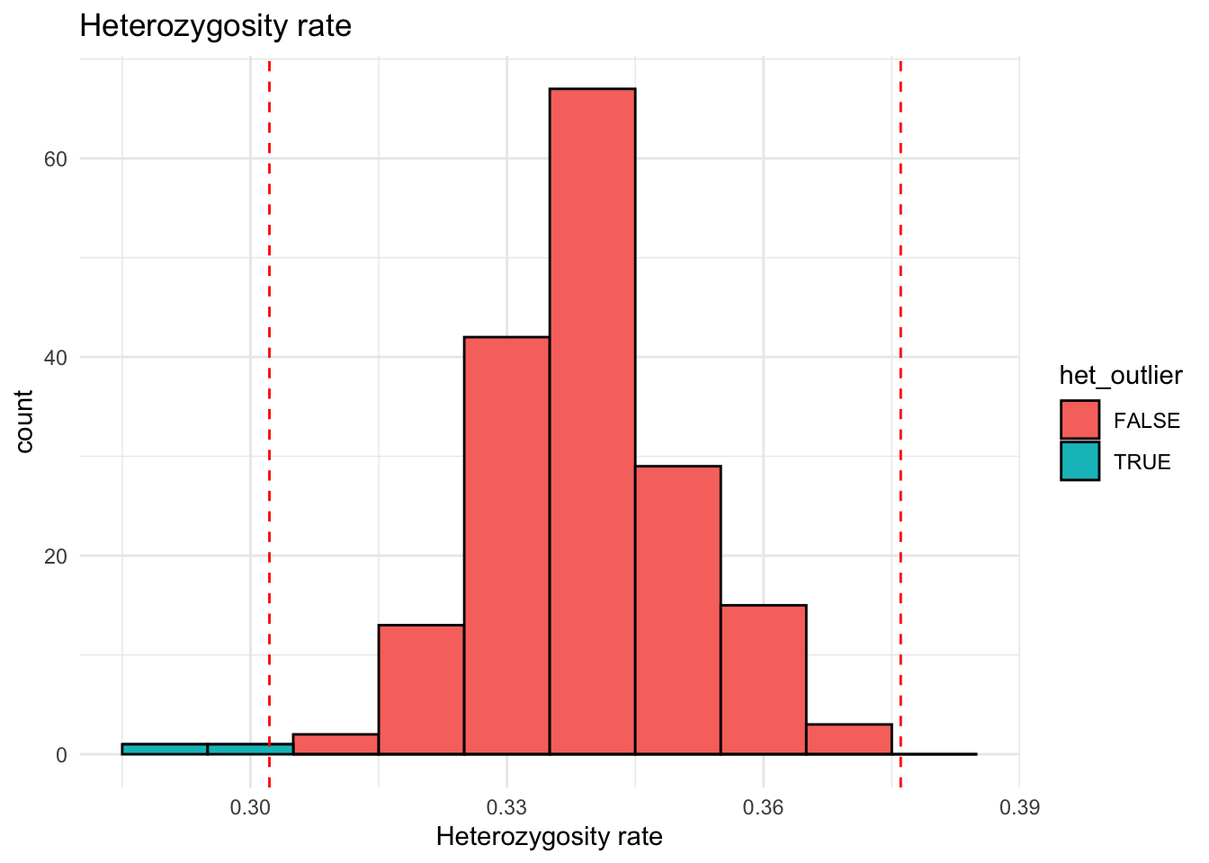

Thresholding

Putting it together: below we (i) filter samples on missingness/heterozygosity, (ii) apply preliminary variant filters (missingness + MAF), (iii) LD‑prune and estimate relatedness (KING) on that prelim set, and later (iv) compute HWE within ancestry‑homogeneous unrelated subsets using the metadata to finalize variant inclusion. This order avoids false HWE failures from population mixture/relatedness. (Anderson et al., 2010)

thr_samp_miss <- 0.02
thr_var_miss <- 0.02
thr_maf <- 0.05
thr_het_z <- 3

keep_sample <- which(samp_miss <= thr_samp_miss & abs(scale(het_rate)) < thr_het_z)
samp.keep.id <- samp.id[keep_sample]

keep_snp_prelim <- which(miss_var <= thr_var_miss & maf >= thr_maf)
snp.prelim.id <- snp.id[keep_snp_prelim]
length(snp.prelim.id)

[1] 18960

SNP correlation structure

max_plot_snps <- 100
ld_snp_ids <- snp.prelim.id[seq_len(max_plot_snps)]

ld_mat <- snpgdsLDMat(
    g,
    sample.id = samp.keep.id,
    snp.id = ld_snp_ids,
    slide = -1,
    method = "corr"
)

Linkage Disequilibrium (LD) estimation on genotypes:
    # of samples: 167
    # of SNPs: 100
    using 1 thread
    method: correlation
LD matrix:    the sum of all selected genotypes (0,1,2) = 9659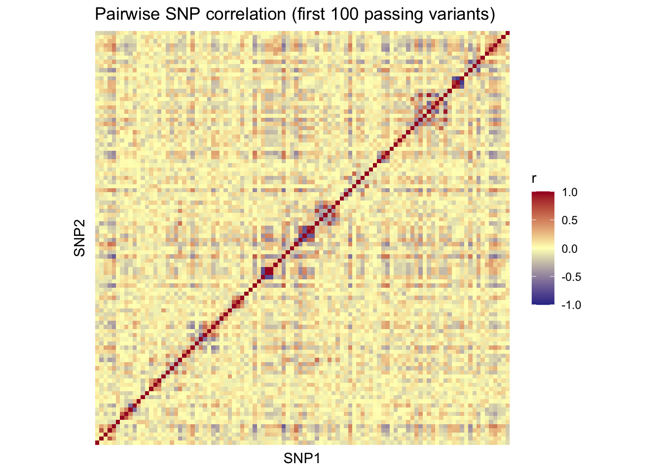

LD pruning

LD pruning removes variants in high LD to yield a subset of approximately independent variants. This is useful for population structure and relatedness estimation, which can be distorted by large blocks of correlated SNPs.

The algorithm works as follows (Zheng et al., 2012):

1. Randomly select a starting position i (start.pos="random"), i=1 if start.pos="first", or i=last if start.pos="last"; and let the current SNP set S={ i };
2. For each right position j from i+1 to n: if any LD between j and k is greater than ld.threshold, where k belongs to S, and both of j and k are in the sliding window, then skip j; otherwise, let S be S + { j };
3. For each left position j from i-1 to 1: if any LD between j and k is greater than ld.threshold, where k belongs to S, and both of j and k are in the sliding window, then skip j; otherwise, let S be S + { j };
4. Output S, the final selection of SNPs.

set.seed(1)
ld_prune <- snpgdsLDpruning(g,
    sample.id = samp.keep.id, 
    snp.id = snp.prelim.id,
    autosome.only = TRUE,
    method = "r",
    slide.max.bp = 500000,
    ld.threshold = sqrt(.1)
)

SNP pruning based on LD:
Excluding 1,040 SNPs (non-autosomes or non-selection)
Excluding 0 SNP (monomorphic: TRUE, MAF: 0.005, missing rate: 0.05)
    # of samples: 167
    # of SNPs: 18,960
    using 1 thread
    sliding window: 500,000 basepairs, Inf SNPs
    |LD| threshold: 0.316228
    method: R
Chrom 1: |====================|====================|
    21.27%, 4,255 / 20,000 (Wed Oct  8 09:36:05 2025)
4,255 markers are selected in total.

snps_pruned <- unlist(ld_prune, use.names = FALSE)

Relatedness

We need to account for relatedness to avoid confounding in PCA and association testing. KING (Kinship‑based INference for GWAS) estimates pairwise kinship robust to population structure (Manichaikul et al., 2010).

1king <- snpgdsIBDKING(g,
                      sample.id = samp.keep.id,
                      snp.id = snps_pruned,
                      type = "KING-robust",
2                      family.id = metadata$FID[match(samp.keep.id, metadata$IID)])

3KINGmat <- GENESIS::kingToMatrix(king)

1

Run KING on our dataset with the filtered samples and LD‑pruned SNPs.

2

Model is robust to misspecifications in population structure.

3

Convert into a kinship matrix we can use for downstream tasks.

Using 167 samples provided

Identifying clusters of relatives...

    154 relatives in 29 clusters; largest cluster = 49

Creating block matrices for clusters...

13 samples with no relatives included

Putting all samples together into one block diagonal matrix

IBD analysis (KING method of moment) on genotypes:
Excluding 15,745 SNPs (non-autosomes or non-selection)
Excluding 0 SNP (monomorphic: TRUE, MAF: NaN, missing rate: NaN)
    # of samples: 167
    # of SNPs: 4,255
    using 1 thread
# of families: 73, and within- and between-family relationship are estimated differently.
Relationship inference in the presence of population stratification.
KING IBD:    the sum of all selected genotypes (0,1,2) = 365234
CPU capabilities:
Wed Oct  8 09:36:05 2025    (internal increment: 65536)

[..................................................]  0%, ETC: ---        
[==================================================] 100%, completed, 0s
Wed Oct  8 09:36:05 2025    Done.

HWE within ancestry groups (metadata + unrelateds)

Under random mating and no technical artifacts, genotype frequencies should follow the familiar proportions under HWE for allele frequency p. A simple check is whether observed counts depart more than sampling noise would predict. In GWAS array data, notable departures often flag lab/array problems rather than biology. Common culprits are poor clustering for one allele, batch effects, or plate swaps (all of which distort heterozygote vs. homozygote balance).

For case-control studies, we compute HWE in controls. True disease associations can produce real departures in cases (e.g., risk allele homozygotes enriched), so filtering on cases risks discarding biological signal. (Anderson et al., 2010)

We will use an exact test for bi‑allelic SNPs. Asymptotic chi‑square tests can mis‑calibrate at low genotype counts or low MAF, while exact tests keep Type I error in check across MAF ranges. (Wigginton et al., 2005; Guo and Thompson, 1992)

Regarding a specific threshold, large studies typically use $p < 10^{−6} as a conservative filter. Smaller studies sometimes use p < 10^{-4}. Because power to detect departures depends on MAF we can consider MAF‑stratified thresholds to avoid over‑penalizing rare variants. (Anderson et al., 2010)

X/sex chromosomes require specific sex‑aware tests (not used here; single autosome). (Anderson et al., 2010)

To avoid the Wahlund effect (heterozygote deficit from pooling distinct ancestries) and non‑independence from relatives, we compute HWE within ancestry‑homogeneous, unrelated subsets. We use KING to define unrelateds and the metadata population labels (ASW, MXL) for grouping.

# Identify unrelateds (3rd‑degree or closer considered related)
km <- KINGmat |> as.matrix()
diag(km) <- 0 
1unrel_ids <- rownames(km)[rowSums(km >= 0.0442, na.rm = TRUE) == 0]
unrel_ids <- intersect(unrel_ids, samp.keep.id)

2grp <- split(unrel_ids, metadata$population[match(unrel_ids, metadata$IID)])

# Exact HWE p-values per group on prelim variants
3p_by_grp <- lapply(grp, function(ids) {
  snpgdsHWE(g, snp.id = snp.prelim.id, sample.id = ids)
})
p_mat <- do.call(cbind, p_by_grp)

4thr_hwe <- 1e-6

# Conservative rule: pass only if all groups pass
5pass_all <- apply(p_mat, 1, function(p) all(is.na(p) | p > thr_hwe))

# Final variant set after HWE
keep_snp <- which(pass_all)
snp.keep.id <- snp.prelim.id[keep_snp]
length(snp.prelim.id)
length(snp.keep.id)

1

Define unrelateds as those with kinship < 0.0442 (3rd-degree or closer) to any other sample.

2

Split unrelateds by population using metadata

3

Compute exact HWE p-values for each group on the preliminary variant set

4

Set a stringent HWE p-value threshold

5

Retain variants that pass HWE in all groups

[1] 18960
[1] 18960

Note that we end up not filtering any variants with this dataset.

Ancestry PCs

With a kinship matrix in hand, we estimate ancestry PCs to use as covariates. PC‑AiR computes PCs on a subset of unrelated individuals and projects relateds onto that space, providing robust structure estimates in the presence of relatedness (Conomos et al., 2015).

1snpgdsClose(g)
2geno_reader <- GWASTools::GdsGenotypeReader(gdsfile)
3geno_data <- GenotypeData(geno_reader)
4pcair_out <- pcair(geno_data,
                   kinobj = KINGmat,
                   divobj = KINGmat,
                   snp.include = snps_pruned,
                   sample.include = samp.keep.id)

1

We need to close the SNPRelate connection before opening with GWASTools

2

Open the GDS file with GWASTools

3

Create a GenotypeData object for analysis

4

Run PC-AiR using the KING kinship matrix to identify unrelateds and compute PCs

Using kinobj and divobj to partition samples into unrelated and related sets

Working with 167 samples

Identifying relatives for each sample using kinship threshold 0.0220970869120796

Identifying pairs of divergent samples using divergence threshold -0.0220970869120796

Partitioning samples into unrelated and related sets...

Unrelated Set: 92 Samples 
Related Set: 75 Samples

Performing PCA on the Unrelated Set...

Predicting PC Values for the Related Set...

Principal Component Analysis (PCA) on genotypes:
Excluding 15,745 SNPs (non-autosomes or non-selection)
Excluding 0 SNP (monomorphic: TRUE, MAF: NaN, missing rate: NaN)
    # of samples: 92
    # of SNPs: 4,255
    using 1 thread
    # of principal components: 32
PCA:    the sum of all selected genotypes (0,1,2) = 201672
CPU capabilities:
Wed Oct  8 09:36:05 2025    (internal increment: 5340)

[..................................................]  0%, ETC: ---        
[==================================================] 100%, completed, 0s
Wed Oct  8 09:36:05 2025    Begin (eigenvalues and eigenvectors)
Wed Oct  8 09:36:05 2025    Done.
SNP Loading:
    # of samples: 92
    # of SNPs: 4,255
    using 1 thread
    using the top 32 eigenvectors
SNP Loading:    the sum of all selected genotypes (0,1,2) = 201672
Wed Oct  8 09:36:05 2025    (internal increment: 42740)

[..................................................]  0%, ETC: ---        
[==================================================] 100%, completed, 0s
Wed Oct  8 09:36:05 2025    Done.
Sample Loading:
    # of samples: 75
    # of SNPs: 4,255
    using 1 thread
    using the top 32 eigenvectors
Sample Loading:    the sum of all selected genotypes (0,1,2) = 163562
Wed Oct  8 09:36:05 2025    (internal increment: 52428)

[..................................................]  0%, ETC: ---        
[==================================================] 100%, completed, 0s
Wed Oct  8 09:36:05 2025    Done.

pcair_tb <- pcair_out$vectors |>
    as_tibble() |>
    bind_cols("IID" = pcair_out$sample.id) |>
    left_join(metadata, by = "IID")

pcair_tb |>
    ggplot(aes(V1, V2, col = population)) +
    geom_point()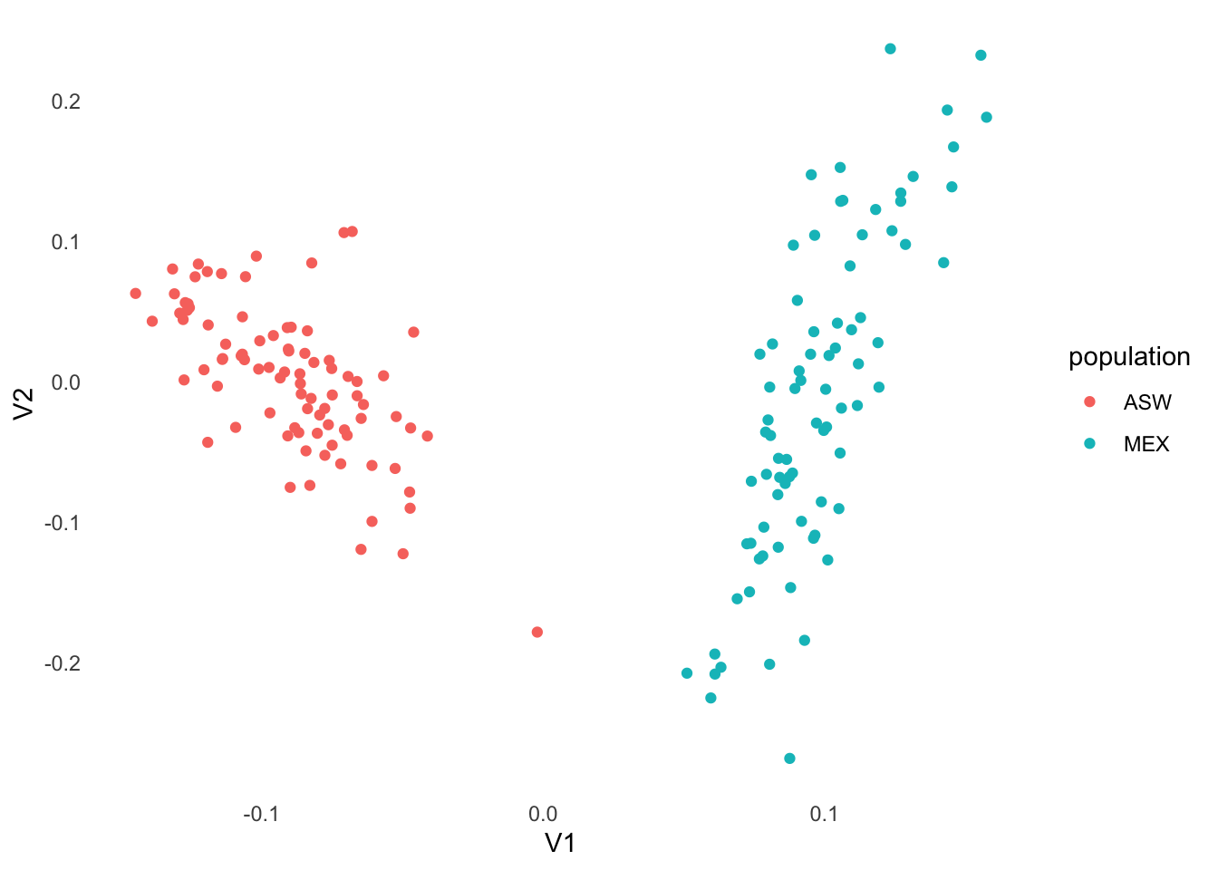

We can use a screeplot to visualize the variance explained by each PC. Depending on where we see an “elbow” in the screeplot, we might choose to include the corresponding PCs in our model.

pcair_out$values |>
    as_tibble() |>
    mutate(PC = row_number()) |>
    ggplot(aes(PC, value)) +
    geom_point() +
    geom_line() +
    scale_x_continuous(breaks = seq(1, 10, by = 1)) +
    labs(title = "Screeplot of PC-AiR eigenvalues", x = "Principal Component", y = "Eigenvalue")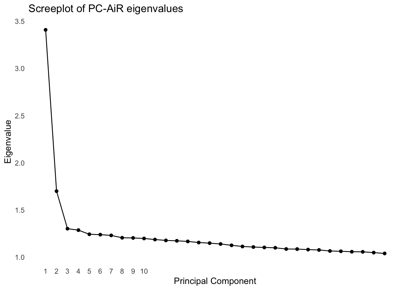

Ancestry‑adjusted relatedness

Now that we have ancestry PCs, we estimate relatedness adjusted for ancestry using PC‑Relate and convert it to a GRM suitable for the null model. Training on the unrelated set stabilizes estimates. (Conomos et al., 2016)

genodata_iter <- GenotypeBlockIterator(geno_data, snpInclude=snps_pruned)

pcrel <- GENESIS::pcrelate(
  gdsobj = genodata_iter,
  pcs = pcair_out$vectors[,1:3],
  training.set = intersect(unrel_ids, pcair_out$sample.id),
  sample.include = samp.keep.id,
)

Using 6 CPU cores

167 samples to be included in the analysis...

Betas for 3 PC(s) will be calculated using 20 samples in training.set...

Running PC-Relate analysis for 167 samples using 4255 SNPs in 1 blocks...

Performing Small Sample Correction...

pcrelMat <- GENESIS::pcrelateToMatrix(pcrel, scaleKin = 2)

Using 167 samples provided

Identifying clusters of relatives...

    167 relatives in 1 clusters; largest cluster = 167

Creating block matrices for clusters...

0 samples with no relatives included

Construct phenotype and merge covariates

For the sake of this demo, we will simulate a quantitative trait with a known genetic effect

set.seed(99)
N <- length(samp.keep.id)
# Use recorded sex from metadata for covariates (single chromosome: no sex-chr analysis needed)
sex <- metadata |>
    filter(IID %in% samp.keep.id) |>
    mutate(sex = case_when(sex == 1 ~ "M",
                           TRUE ~ "F")) |>
    pull(sex)

# Choose one moderately frequent SNP and simulate a quantitative trait with a planted effect
maf_keep <- maf[snp.keep.id]
ix <- which(!is.na(maf_keep) & maf_keep > 0.2 & maf_keep < 0.3)[1]

G1 <- GWASTools::getGenotypeSelection(geno_data, snpID = snp.keep.id[ix], scanID = samp.keep.id)
G1 <- as.numeric(G1) 
y <- as.numeric(0.4* scale(G1) + 0.05 * (sex == "M") + rnorm(N))

We now have a phenotype vector y and covariates. We need to construct a ScanAnnotationDataFrame object for the null model fitting.

pcs_df <- data.frame(
  scanID = pcair_out$sample.id,
  PC1 = pcair_out$vectors[, 1],
  PC2 = pcair_out$vectors[, 2],
  PC3 = pcair_out$vectors[, 3]
)

scanDF <- dplyr::left_join(
  data.frame(scanID = samp.keep.id, y = y, sex = sex),
  pcs_df,
  by = "scanID"
)

scanAnnot2 <- GWASTools::ScanAnnotationDataFrame(scanDF)

Step 3: Modeling

Null model

We first fit the mixed model under the null hypothesis that each SNP has no effect. The null includes covariates (age, sex, ancestry PCs) and a random genetic effect capturing relatedness; it does not include per‑SNP fixed effects.

The model:

y = X\beta + g + \epsilon

Where y is the phenotype, X\beta are fixed‑effect covariates, g \sim \mathcal{N}(0, \sigma^2_g K) is the random genetic effect with relatedness matrix K, and \epsilon \sim \mathcal{N}(0, \sigma^2_e I) is residual error.

Notes on estimation

• Covariance under the null: \operatorname{Var}(y) = V = \sigma^2_e I + \sigma^2_g K.
• We pass an ancestry‑adjusted GRM from PC‑Relate
  • This yields diagonals near 1 (via pcrelateToMatrix(scaleKin=2)) and controls for population structure in kinship estimation
• Fixed effects (GLS) estimator given variance components: \hat{\beta} = (X^\top V^{-1} X)^{-1} X^\top V^{-1} y.
• Variance components for Gaussian outcomes are estimated by REML.
• Heritability estimate: h^2 = \sigma^2_g/(\sigma^2_g + \sigma^2_e).

nullmod <- GENESIS::fitNullModel(
    scanAnnot2,
    outcome = "y",
    covars = c("sex", "PC1", "PC2", "PC3"),
    cov.mat = pcrelMat, family = "gaussian"
)

Computing Variance Component Estimates...

Sigma^2_A     log-lik     RSS

[1]    0.5717426    0.5717426 -243.7704375    1.0182557
[1]    0.1884426    0.8753057 -242.1753414    1.0461782
[1]    0.2420265    0.8685482 -242.1442635    1.0026855
[1]    0.2408589    0.8726307 -242.1442236    1.0000083
[1]    0.2411044    0.8724022 -242.1442228    1.0000000

nullmod$varComp

        V_A V_resid.var 
  0.2411044   0.8724022 

varComp reports the variance components from the mixed model. The entry V_A is the additive‑genetic variance captured by our GRM (PC‑Relate), and V_resid.var is the residual variance after adjusting for age, sex, and ancestry PCs. A convenient summary is the mixed‑model heritability on this working scale, h^2 = \frac{V_A}{V_A + V_{resid}}

varc <- nullmod$varComp
h2 <- unname(varc["V_A"] / sum(varc))

tibble::tibble(
  component = c("V_A", "V_resid", "h2_mixed_model"),
  value = c(varc["V_A"], varc["V_resid.var"], h2)
)

# A tibble: 3 × 2
  component      value
  <chr>          <dbl>
1 V_A            0.241
2 V_resid        0.872
3 h2_mixed_model 0.217

Association testing

We now test each SNP for association with the phenotype using a score test. The score test is computationally efficient because it only requires fitting the null model once, rather than refitting for each SNP as in a Wald or likelihood ratio test.

# Genotype iterator (block-wise scan of all SNPs kept by QC)
it <- GWASTools::GenotypeBlockIterator(
    geno_data, 
    snpInclude = snp.keep.id, 
    snpBlock = 5000
)
assoc <- GENESIS::assocTestSingle(it, null.model = nullmod, test = "Score")

Using 6 CPU cores

res <- data.frame(
    SNP = assoc$variant.id,
    CHR = as.numeric(assoc$chr),
    BP = assoc$pos,
    P = assoc$Score.pval,
    BETA = assoc$Est,
    SE = assoc$Est.SE
)

Step 4: Post‑GWAS

Extracting results

        SNP    BP       BETA        SE            P
6         6     6  0.8396265 0.1568205 8.600221e-08
4628   4892  4892 -0.5765968 0.1501810 1.233630e-04
9363   9895  9895 -0.5772324 0.1532537 1.655421e-04
1796   1878  1878 -0.5223076 0.1415787 2.249887e-04
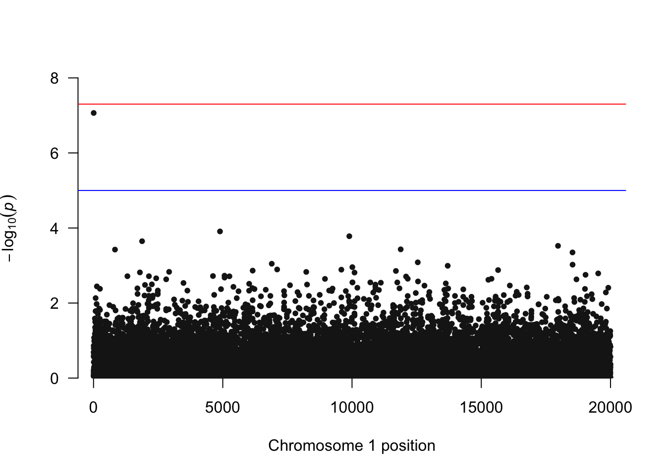
17050 17968 17968  0.4745057 0.1312115 2.987953e-04

[1] 6

Note that our top SNP is the one we simulated to have an effect.

Manhattan plot

We visualize the genome‑wide p-values using a Manhattan plot. The blue line indicates a p-value threshold of 1 \times 10^{-5}. Note that this is equivalent to a Bonferroni correction for 5,000 independent tests. The red line at 5 \times 10^{-8} is a common genome‑wide significance threshold for GWAS, though it is conservative for smaller studies or those with fewer variants.

# qqman expects columns named: CHR, BP, SNP, P
qqman::manhattan(
  res,
  chr = "CHR", bp = "BP", snp = "SNP", p = "P",
  suggestiveline = -log10(1e-5)
)

QQ Plot

We compare observed p‑values to the null expectation to assess calibration. Few true signals should deviate strongly.

qqman::qq(res$P)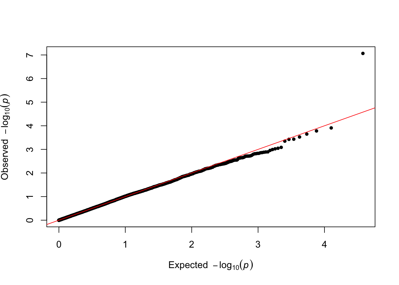

Genomic-control inflation factor

The genomic-control inflation factor is a single-number summary (\lambda_{GC}) of how inflated or conservative the genome‑wide test statistics are relative to the null. Values near 1 indicate well‑calibrated tests, >1 suggests inflation (e.g., population structure, relatedness, batch), <1 suggests conservative/underpowered tests

For 1‑df tests, the null statistic follows \chi^2_1, whose median is qchisq(0.5, 1) \approx 0.456. We will convert our p‑values to \chi^2 statistics T_i = \texttt{qchisq}(1 − p_i, df = 1). Then \lambda_{GC} = \text{median}(T_i) / m_0.

lambda_gc <- median(stats::qchisq(1 - res$P, df = 1), na.rm = TRUE) / 0.456
lambda_gc

[1] 0.9851403

Cleanup

When done, close the GDS connection

GWASTools::close(geno_reader)

When to use a different tool?

• For very large datasets (e.g., UK Biobank), specialized tools like BOLT-LMM, REGENIE, or SAIGE may be more efficient
• For binary traits, consider tools that handle case-control imbalance and relatedness effectively, such as SAIGE
• For rare variant analysis, consider burden tests or SKAT implemented in packages like SKAT or seqMeta

Further reading

• Population Structure and Relatedness Inference using the GENESIS Package
• Genetic Association Testing using the GENESIS Package
• Using PLINK for GWAS

Session Info

sessionInfo()

R version 4.5.1 (2025-06-13)
Platform: aarch64-apple-darwin20
Running under: macOS Tahoe 26.0.1

Matrix products: default
BLAS:   /Library/Frameworks/R.framework/Versions/4.5-arm64/Resources/lib/libRblas.0.dylib 
LAPACK: /Library/Frameworks/R.framework/Versions/4.5-arm64/Resources/lib/libRlapack.dylib;  LAPACK version 3.12.1

locale:
[1] C.UTF-8/C.UTF-8/C.UTF-8/C/C.UTF-8/C.UTF-8

time zone: America/New_York
tzcode source: internal

attached base packages:
[1] stats     graphics  grDevices datasets  utils     methods   base     

other attached packages:
 [1] readr_2.1.5         dplyr_1.1.4         ggplot2_3.5.2      
 [4] qqman_0.1.9         GWASTools_1.54.0    Biobase_2.68.0     
 [7] BiocGenerics_0.54.0 generics_0.1.4      GENESIS_2.38.0     
[10] SNPRelate_1.42.0    gdsfmt_1.44.1      

loaded via a namespace (and not attached):
  [1] Rdpack_2.6.4            DBI_1.2.3               gridExtra_2.3          
  [4] sandwich_3.1-1          rlang_1.1.6             magrittr_2.0.3         
  [7] SeqVarTools_1.46.0      compiler_4.5.1          RSQLite_2.4.3          
 [10] mgcv_1.9-3              reshape2_1.4.4          vctrs_0.6.5            
 [13] stringr_1.5.1           quantreg_6.1            pkgconfig_2.0.3        
 [16] shape_1.4.6.1           crayon_1.5.3            fastmap_1.2.0          
 [19] backports_1.5.0         XVector_0.48.0          labeling_0.4.3         
 [22] utf8_1.2.6              rmarkdown_2.29          tzdb_0.5.0             
 [25] UCSC.utils_1.4.0        nloptr_2.2.1            MatrixModels_0.5-4     
 [28] purrr_1.0.4             bit_4.6.0               xfun_0.52              
 [31] glmnet_4.1-10           jomo_2.7-6              logistf_1.26.1         
 [34] cachem_1.1.0            GenomeInfoDb_1.44.3     jsonlite_2.0.0         
 [37] blob_1.2.4              pan_1.9                 BiocParallel_1.42.2    
 [40] broom_1.0.8             parallel_4.5.1          R6_2.6.1               
 [43] stringi_1.8.7           RColorBrewer_1.1-3      boot_1.3-31            
 [46] DNAcopy_1.82.0          rpart_4.1.24            lmtest_0.9-40          
 [49] GenomicRanges_1.60.0    Rcpp_1.1.0              iterators_1.0.14       
 [52] knitr_1.50              zoo_1.8-14              IRanges_2.42.0         
 [55] igraph_2.1.4            Matrix_1.7-3            splines_4.5.1          
 [58] nnet_7.3-20             tidyselect_1.2.1        viridis_0.6.5          
 [61] yaml_2.3.10             codetools_0.2-20        curl_6.2.3             
 [64] plyr_1.8.9              lattice_0.22-7          tibble_3.3.0           
 [67] quantsmooth_1.74.0      withr_3.0.2             evaluate_1.0.3         
 [70] survival_3.8-3          Biostrings_2.76.0       pillar_1.11.0          
 [73] BiocManager_1.30.26     mice_3.18.0             renv_1.1.5             
 [76] foreach_1.5.2           stats4_4.5.1            reformulas_0.4.1       
 [79] vroom_1.6.5             S4Vectors_0.46.0        hms_1.1.3              
 [82] scales_1.4.0            minqa_1.2.8             calibrate_1.7.7        
 [85] GWASExactHW_1.2         glue_1.8.0              tools_4.5.1            
 [88] data.table_1.17.4       lme4_1.1-37             SparseM_1.84-2         
 [91] cowplot_1.1.3           grid_4.5.1              tidyr_1.3.1            
 [94] rbibutils_2.3           nlme_3.1-168            formula.tools_1.7.1    
 [97] GenomeInfoDbData_1.2.14 cli_3.6.5               SeqArray_1.48.3        
[100] viridisLite_0.4.2       gtable_0.3.6            digest_0.6.37          
[103] operator.tools_1.6.3    farver_2.1.2            memoise_2.0.1          
[106] htmltools_0.5.8.1       lifecycle_1.0.4         httr_1.4.7             
[109] mitml_0.4-5             bit64_4.6.0-1           MASS_7.3-65            

References

Anderson,C.A. et al. (2010) Data quality control in genetic case–control association studies. Nature Protocols, 5, 1564–1573.

Conomos,M.P. et al. (2016) Model-free estimation of recent genetic relatedness. The American Journal of Human Genetics, 98, 127–148.

Conomos,M.P. et al. (2015) Robust inference of population structure for ancestry prediction and correction of stratification in the presence of relatedness. Genetic Epidemiology, 39, 276–293.

Guo,S.W. and Thompson,E.A. (1992) Performing the exact test of Hardy–Weinberg proportion for multiple alleles. Biometrics, 48, 361–372.

Manichaikul,A. et al. (2010) Robust relationship inference in genome-wide association studies. Bioinformatics, 26, 2867–2873.

The International HapMap 3 Consortium (2010) Integrating common and rare genetic variation in diverse human populations. Nature, 467, 52–58.

The International HapMap Consortium (2005) A haplotype map of the human genome. Nature, 437, 1299–1320.

Wigginton,J.E. et al. (2005) A note on exact tests of Hardy–Weinberg equilibrium. The American Journal of Human Genetics, 76, 887–893.

Zheng,X. et al. (2012) A high-performance computing toolset for relatedness and principal component analysis of SNP data. Bioinformatics, 28, 3326–3328.