.jpg)
| name | team | league | hits | at_bats | early_avg | final_avg |
|---|---|---|---|---|---|---|
| Roberto Clemente | Pitts | NL | 18 | 45 | 0.400 | 0.346 |
| Frank Robinson | Balt | AL | 17 | 45 | 0.378 | 0.298 |
| Frank Howard | Wash | AL | 16 | 45 | 0.356 | 0.276 |
| Jay Johnstone | Cal | AL | 15 | 45 | 0.333 | 0.222 |
| Ken Berry | Chi | AL | 14 | 45 | 0.311 | 0.273 |
| Jim Spencer | Cal | AL | 14 | 45 | 0.311 | 0.270 |
Lecture 06: Prediction models in genetics
PUBH 8878, Statistical Genetics
Inference vs Prediction
- So far, we have talked about estimation of certain quantities of interest
- p: Allele frequencies
- \beta: Association effect sizes
- \pi: Ancestry proportions
Inference vs Prediction
- Some tasks, however, focus on predicting outcomes rather than estimating parameters.
- Disease risk classification (polygenic risk scores, case vs control)
- Absolute/lifetime risk and time-to-event predictions
- Drug response/toxicity prediction
Inference vs Prediction
While not mutually exclusive, these tasks require different approaches and metrics
- Association
- Goal: identify variants related to trait.
- Target: low FDR/valid inference, effect estimates with SEs.
- Tools: single‑variant tests, LMMs, fine‑mapping
- Prediction
- Goal: accurate out‑of‑sample trait/risk estimates.
- Target: minimize expected loss (MSE, log loss)
- Tools: penalized GLMs, BLUP/GBLUP, ensembles, NNs
Bait and Switch
Today we will be talking about baseball! (Briefly)

Prediction in baseball
- Task: predict a later‑season batting rate using the first 45 at‑bats for each player
Our data
Estimating batting averages
- If we assume that each player’s batting average comes from a binomial distribution, then the MLE is the sample proportion \hat{p_i} = h_i/n_i
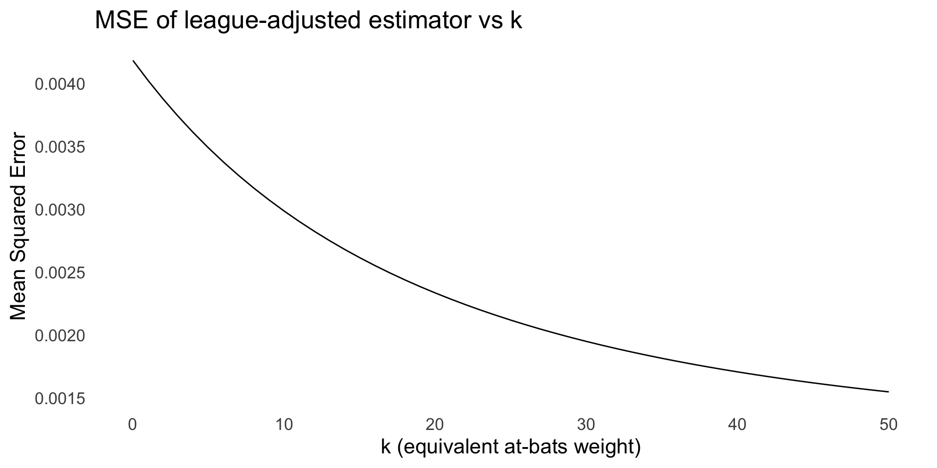
- A different approach is to use a beta prior centered at the league average
- The prior is p_i \sim \mathrm{Beta}(\alpha, \beta) with \alpha = \bar p \kappa and \beta = (1 - \bar p)\kappa, where \bar p is the league average
league_avg <- mean(batting_averages$hits / batting_averages$at_bats)

k_grid <- tibble(k = seq(0, 50, by = 1))

batting_avg_long <- tidyr::crossing(batting_averages, k_grid) |>
    mutate(alpha = league_avg * k,
           beta  = (1 - league_avg) * k,
           p_k   = (alpha + hits) / (alpha + beta + at_bats),
           estimator = paste0("k=", k)
           )
Note: k=0 corresponds to the (improper) Beta(0,0) prior; in this limit the posterior mean reduces to the MLE h/n.
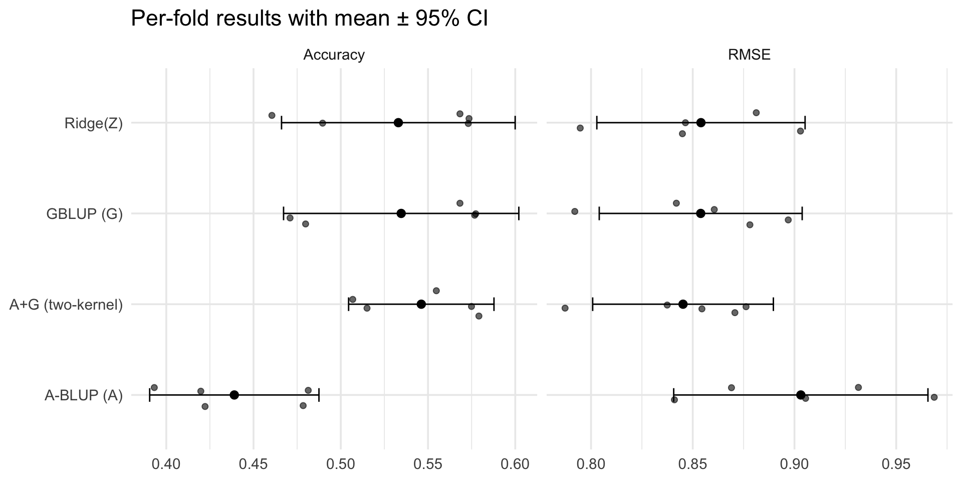
Prediction performance
Shrinkage visualization
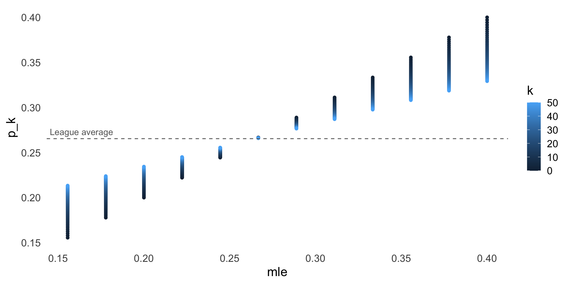
What are we doing here?
- Our beta-binomial model makes an assumption that players regress toward the league average
- More statistically, we are assuming that the true batting averages are drawn from a common prior distribution centered at the league average
Back to genetics
- The same principles apply when performing prediction in genetics
- Many problems involve a large number of genetic variants (p) and relatively small sample sizes (n)
- When p > n, linear regression is singular
- This means the design matrix does not have full rank, leading to non-unique solutions
- We solve this by imposing strong structure (assumptions) on effects
p >> n: structural assumptions we use
- Sparsity: most variant effects are 0 (lasso, debiased lasso for inference)
- Gaussian shrinkage: many small effects (ridge, BLUP/GBLUP, PRS-CS)
- Low-rank/latent structure: factors, PCs, random effects (LMMs)
- Smoothness/blocks: genomic locality/LD (fused/TV penalties, windowed methods)
- Hybrid/empirical Bayes: estimate prior from data + partial pooling
Examples of Shrinkage/Sparse Estimators
- Ridge regression
- Lasso regression
- Elastic net
- Bayesian linear regression with Gaussian priors
- BLUP/GBLUP in genetics
- DESeq2 (transcriptomics)
What is BLUP?
- BLUP = Best Linear Unbiased Prediction of random effects in a mixed model.
- Model (K-based view): y = \mu\,\mathbf 1 + g + \varepsilon, with g \sim \mathcal N(0, \sigma_g^2 K) and \varepsilon \sim \mathcal N(0, \sigma_e^2 I).
- Equivalent marker-effects view: y = \mu\,\mathbf 1 + Z\beta + \varepsilon with \beta\sim\mathcal N(0,\sigma_\beta^2 I_m); then g=Z\beta and \operatorname{Cov}(g)=\sigma_\beta^2 ZZ^\top = \sigma_g^2 K with \sigma_g^2 = m\,\sigma_\beta^2 when K=ZZ^\top/m.
- BLUP shrinks random effects toward 0; predictions \hat y shrink toward the mean \mu.
- As \sigma_g^2/\sigma_e^2 \to 0, predictions shrink to the mean.
- Pedigree-based BLUP: use K = A, the expected relatedness matrix from pedigrees.
- Genomic BLUP: use K = G, the realized similarity matrix from marker data.
Relationship matrices A and G
- Pedigree A:
- A_{ij} = 2\,\phi_{ij}, where \phi_{ij} is the kinship (coancestry) coefficient; A_{ii} = 1 + F_i (with inbreeding F_i).
- Requires accurate pedigrees.
- Genomic G (unified with ridge via standardized markers):
- Build a standardized marker matrix Z by centering each SNP by its allele frequency and scaling by its standard deviation.
- 0/1 SNPs: Z_{ij} = (X_{ij} - p_j)/\sqrt{p_j(1-p_j)}.
- 0/1/2 SNPs: Z_{ij} = (X_{ij} - 2p_j)/\sqrt{2p_j(1-p_j)}.
- Set G = ZZ^\top / m with m markers; then \operatorname{E}[\operatorname{diag}(G)] \approx 1.
- Build a standardized marker matrix Z by centering each SNP by its allele frequency and scaling by its standard deviation.
Ridge, Kernel Ridge, and GBLUP: One Model, Three Views
Setup and assumptions
- Let Z\in\mathbb R^{n\times m} be the standardized marker matrix: each column centered and scaled so \mathbf 1^\top Z = 0 and \mathrm{Var}(Z_{\cdot j})\approx 1.
- Define the genomic similarity K = ZZ^\top/m. Then K\,\mathbf 1 = 0 and \operatorname{E}[\operatorname{diag}(K)] \approx 1.
- With an intercept, y=\mu\,\mathbf 1 + Z\beta + \varepsilon, the centering implies the intercept decouples and \hat\mu = \bar y (in cross‑validation, use the training‑fold mean \bar y_{\text{train}}). Write \tilde y = y - \bar y\,\mathbf 1.
Ridge, Kernel Ridge, and GBLUP: One Model, Three Views
Primal ridge (marker‑effects view)
- Objective: \min_\beta\; \tfrac12\Vert \tilde y - Z\beta\Vert_2^2 + \tfrac\lambda2\Vert\beta\Vert_2^2.
- Closed form: \displaystyle \hat\beta = (Z^\top Z + \lambda I_m)^{-1} Z^\top \tilde y, and predictions \hat y = \bar y\,\mathbf 1 + Z\hat\beta.
- Bayesian view: \beta\sim\mathcal N(0,\sigma_\beta^2 I_m), \varepsilon\sim\mathcal N(0,\sigma_e^2 I_n) gives \lambda = \sigma_e^2/\sigma_\beta^2.
Ridge, Kernel Ridge, and GBLUP: One Model, Three Views
Dual (kernel) ridge
- Work in the n‑dimensional span of samples: solve \hat\alpha = (K + \lambda_K I_n)^{-1}\tilde y,\qquad \hat y = \bar y\,\mathbf 1 + K\hat\alpha.
- Equivalence identity: (Z^\top Z + \lambda I_m)^{-1} Z^\top = Z^\top (ZZ^\top + \lambda I_n)^{-1}. Hence \hat\beta = Z^\top\hat\alpha and Z\hat\beta = K\hat\alpha ⇒ identical predictions when hyperparameters match.
- Hyperparameter mapping with K=ZZ^\top/m: set \boxed{\;\lambda_K = \lambda/m\;}\; (equivalently \lambda = m\,\lambda_K).
Ridge, Kernel Ridge, and GBLUP: One Model, Three Views
BLUP (mixed‑model view)
- Model: y = \mu\,\mathbf 1 + g + \varepsilon, with g\sim\mathcal N(0,\sigma_g^2 K) and \varepsilon\sim\mathcal N(0,\sigma_e^2 I_n); let V = \sigma_g^2 K + \sigma_e^2 I_n.
- GLS intercept: \hat\mu = (\mathbf 1^\top V^{-1}\mathbf 1)^{-1}\,\mathbf 1^\top V^{-1} y. Because K\,\mathbf 1 = 0, V\,\mathbf 1 = \sigma_e^2\mathbf 1 ⇒ \hat\mu = \bar y.
- BLUP of genetic values: \hat g = \sigma_g^2 K V^{-1}(y - \hat\mu\,\mathbf 1) = K\big(K + (\sigma_e^2/\sigma_g^2) I_n\big)^{-1}(y - \hat\mu\,\mathbf 1). This is kernel ridge on K with \boxed{\;\lambda_K = \sigma_e^2/\sigma_g^2\;}. Predictions are \hat y = \hat\mu\,\mathbf 1 + \hat g.
- Marker‑BLUP equivalence: if \beta\sim\mathcal N(\,0,\,\sigma_\beta^2 I_m), then g=Z\beta\sim\mathcal N(0,\sigma_g^2 K) with \sigma_g^2 = m\,\sigma_\beta^2 (since \operatorname{Var}(Z\beta)=\sigma_\beta^2 ZZ^\top = m\sigma_\beta^2 K). Thus \lambda = \sigma_e^2/\sigma_\beta^2 and \lambda_K = \sigma_e^2/\sigma_g^2 satisfy \lambda = m\,\lambda_K.
Ridge, Kernel Ridge, and GBLUP: One Model, Three Views
Out‑of‑sample prediction
- New individual with standardized genotype z_*\in\mathbb R^m:
- Primal: \hat y_* = \hat\mu + z_*^\top\hat\beta.
- Kernel: form k_* = z_* Z^\top / m and use \hat y_* = \hat\mu + k_*\hat\alpha.
- Shapes: Z_{\text{train}}\in\mathbb R^{n\times m}, z_*\in\mathbb R^m, so k_*\in\mathbb R^n and \alpha\in\mathbb R^n solves (K_{\text{train}}+\lambda_K I)\alpha = y_{\text{train}} - \hat\mu\,\mathbf 1.
Ridge, Kernel Ridge, and GBLUP: One Model, Three Views
Computational notes
- Choose the algebra that fits the dimension: primal solves a m\times m system; dual/kernel solves an n\times n system. When m\gg n, the kernel view is cheaper; when n\gg m, the primal view is cheaper. Conjugate‑gradient or Cholesky apply in either view.
- ABLUP uses K=A (often exploited via sparse A^{-1} in mixed‑model equations); GBLUP uses dense K=G.
Prediction for crop yield
- Consider the problem of predicting grain yield for different wheat lines across multiple environments
- We are interested in modeling the genetic and environmental effects on yield
Dataset at a glance
- Lines: 599 historical wheat lines
- Environments: 4 mega-environments (columns in Y)
- Phenotype (Y): average grain yield (one column per environment)
- Markers (X): (0/1 after QC + imputation)
- Pedigree (A): 599×599 additive relationship from multi-generation pedigree
Breeding context: what are we predicting?
- A “line” = inbred or DH line to be advanced or discarded; objective is to predict its genetic value (GEBV) for yield.
- “Environment (Env)” = location-year-management combination. Yield varies by Env and by G×E (line×environment interaction)
- Target Population of Environments (TPE): we want models that generalize to the environments we care about
Cross‑validation that matches breeding decisions
- Use line‑wise folds so the same line never appears in both train and test.
- For multi‑environment data:
- Goal “new line, known environments” \to mask whole lines across all environments in test.
- Goal “known lines, new environment” \to environment‑wise holdouts and G×E models.
Loading data
Looking at our data
     wPt.0538 wPt.8463 wPt.6348
[1,]        0        1        1
[2,]        1        1        1
[3,] 1 1 1 1 2 4 5
775 1.6716295 -1.7274699 -1.8902848 0.0509159
2166 -0.2527028 0.4095224 0.3093855 -1.7387588
2167 0.3418151 -0.6486263 -0.7995592 -1.0535691 775 2166 2167
775 1.9698 0.5742 0.5742
2166 0.5742 1.9930 1.9930
2167 0.5742 1.9930 1.9966Standardizing markers
- 1
- Calculate allele frequencies per marker
- 2
- Calculate standard deviations for each marker
- 3
- Standardize markers into Z
- 4
- Build genomic relationship matrix G = ZZ^\top / m
- 5
- Normalize A and G
Because columns of Z are mean‑zero and have variance near 1, K=ZZ^\top/m has \operatorname{mean}(\operatorname{diag} K)\approx 1. Dividing A and G by their mean diagonal sets that target exactly and places \sigma_g^2 on a comparable scale across kernels.
Cross-validation folds
- Create a function to generate cross-validation folds
- If we have multiple observations for the same line, ensure they are in the same fold
- Naming note: here
Kdenotes the number of folds; elsewhere K denotes a kernel/relationship matrix. Context distinguishes them.
Metrics functions
metrics <- function(obs, pred) {
  accuracy <- suppressWarnings(cor(obs, pred))
  rmse <- sqrt(mean((obs - pred)^2))
  c(Accuracy = accuracy, RMSE = rmse)
}

by_fold_metrics <- function(y, pred, fold, model_label){
  idx <- split(seq_along(y), fold)
  acc <- sapply(idx, function(ii) suppressWarnings(cor(y[ii], pred[ii])))
  rmse <- sapply(idx, function(ii) sqrt(mean((y[ii] - pred[ii])^2)))
  tibble(Model = model_label, Fold = seq_along(idx), Accuracy = acc, RMSE = rmse)
}- Create functions to compute metrics
Ridge regression
cv_ridge_Z <- function(y, Z, fold, inner_nfolds = 5){
  K <- max(fold)
  pred <- rep(NA_real_, length(y))
  lambda <- numeric(K)
  for(k in seq_len(K)){
    tr <- fold != k; te <- !tr
    fit <- cv.glmnet(Z[tr, , drop = FALSE], y[tr],
                     alpha = 0, standardize = FALSE, intercept = TRUE,
                     nfolds = inner_nfolds)
    pred[te] <- as.numeric(predict(fit, newx = Z[te, , drop = FALSE], s = "lambda.min"))
    lambda[k] <- fit$lambda.min
  }
  list(pred = pred, lambda = lambda)
}- Create a function for ridge regression using
cv.glmnet - Uses
Z, the standardized marker matrix
A/G-BLUP Models
cv_bglr_kernel <- function(y, K, fold, nIter = 6000, burnIn = 1000){
  pred <- rep(NA_real_, length(y))
  for(k in seq_len(max(fold))){
    ytr <- y; ytr[fold == k] <- NA
    fit <- BGLR(y = ytr, ETA = list(list(K = K, model = "RKHS")),
                nIter = nIter, burnIn = burnIn, verbose = FALSE)
    pred[fold == k] <- fit$yHat[fold == k]
  }
  list(pred = pred)
}- Use
BGLRfor kernel ridge regression with a given kernel matrix - The
"RKHS"option directs BGLR to fit a kernel ridge model with covariance \sigma_g^2 K, so shrinkage follows the supplied similarity matrix
A+G-BLUP Models
cv_bglr_AplusG <- function(y, A, G, fold, nIter = 6000, burnIn = 1000){
  pred <- rep(NA_real_, length(y))
  for(k in seq_len(max(fold))){
    ytr <- y; ytr[fold == k] <- NA
    fit <- BGLR(y = ytr,
                ETA = list(list(K = A, model = "RKHS"),
                           list(K = G, model = "RKHS")),
                nIter = nIter, burnIn = burnIn, verbose = FALSE)
    pred[fold == k] <- fit$yHat[fold == k]
  }
  list(pred = pred)
}- Combine pedigree and genomic relationship matrices in a two-kernel model
- This allows modeling both additive genetic effects from pedigree and genomic information
# A tibble: 4 × 5
  Model            avg_acc sd_acc avg_rmse sd_rmse
  <chr>              <dbl>  <dbl>    <dbl>   <dbl>
1 A+G (two-kernel)   0.546 0.0336    0.845  0.0358
2 A-BLUP (A)         0.439 0.0391    0.903  0.0503
3 GBLUP (G)          0.535 0.0543    0.854  0.0402
4 Ridge(Z)           0.533 0.0539    0.854  0.0412
Results