Lecture 07: False Discovery Rates
PUBH 8878, Statistical Genetics
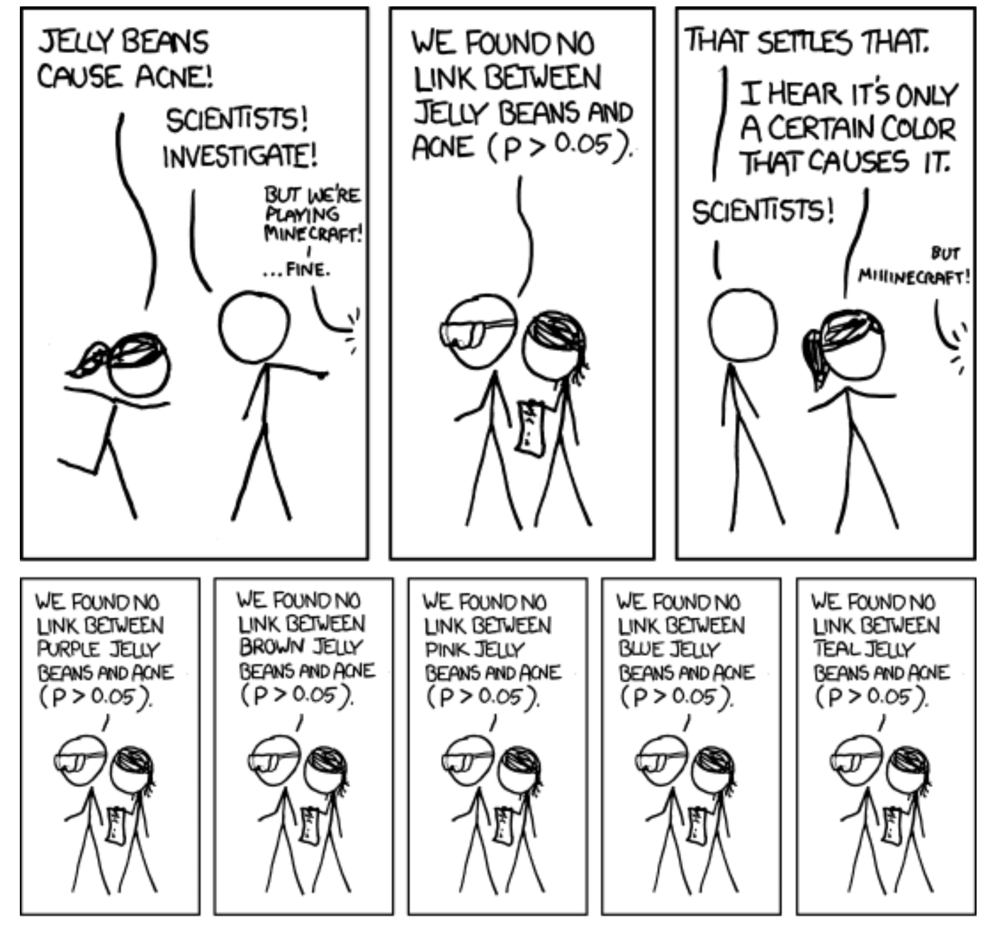
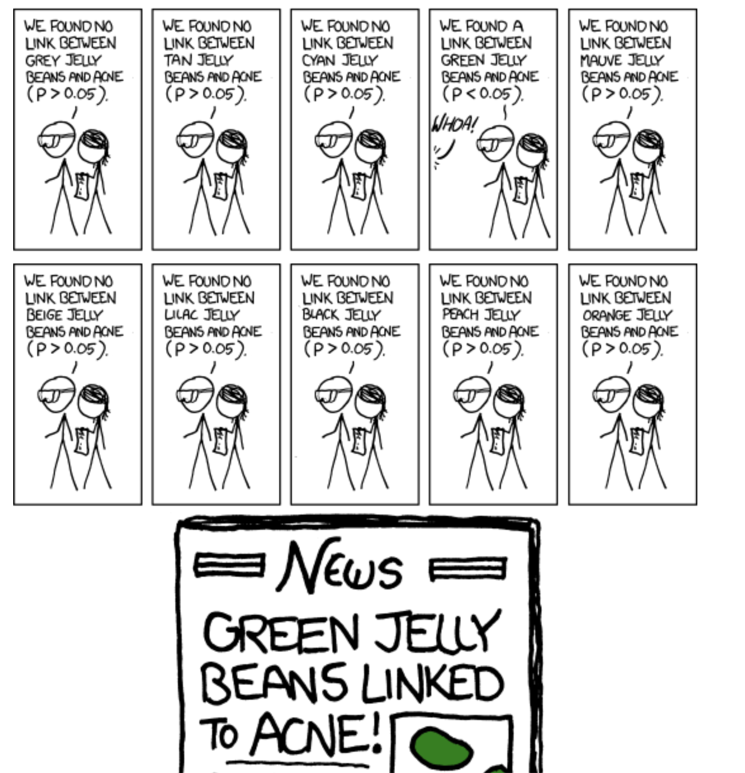
Obligatory XKCD
Problem Set-up
- Consider a GWAS where \(m\) SNPs are tested for association with a trait of interest
- For SNP \(i\), Let \(\delta\) be a unobserved random variable where
\[ \delta_i = \begin{cases} 0 \text{ if the i'th hypothesis is a true null} \\ 1 \text{ if the alternative is true} \end{cases} \]
- Based on some rule, we observe \(r_i\), where
\[ r_i = \begin{cases} 0 \text{ if we fail to reject the i'th hypothesis} \\ 1 \text{ if we reject the i'th hypothesis} \end{cases} \]
Problem Set-up
- For each SNP, given our data, we compute a test statistic \(z_i\)
- We will reject hypothesis \(i\) if \(z_i \in A\), where \(A\) is some rejection region
- Let \(R\) be the total number of rejections, where \(R = \sum_{i=1}^m r_i\)
- Let \(T, V\) be the total number of true and false discoveries respectively, where
\[ T = \sum_{i=1}^m r_i \delta_i, \qquad V = \sum_{i=1}^m r_i (1-\delta_i) \]
- The Family Wise Error Rate (FWER) is the probably that we have at least one false discovery, or \(\text{Pr}(V \geq 1)\)
- The False Discovery Proportion is \(Q = \frac{V}{R}\), where \(Q=0\) if \(R=0\)
Problem Set-up
- Note that \(Q\) is not observable!
- \(V\) is unknown as \(\delta\) is unobservable
- There exist a variety of methods to estimate \(Q\)
Two Preliminaries
- Distribution of \(p\)-values
- Generating a Random Variable with a desired distribution
Distribution of \(p\)-values
- Let \(X \in \mathbb{R}\) be a random variable with pdf \(f_X(x) = \frac{d}{dx}F(x)\)
- Let \(y = F(x)\) such that \(x = F^{-1}(y)\)
- Via theory of transformations, we achieve for \(y \in (0, 1)\)
\[ f_Y(y) = f_X\left(F^{-1}(y)\right)\left| \frac{dF^{-1}(y)}{dy}\right| \]
- Let \(x = F^{-1}(y)\). Then, \(y = F(x)\), and,
\[\begin{align*} \left| \frac{dF^{-1}(y)}{dy}\right| = \frac{dx}{dF(x)} = \frac{dx}{f_X(x) dx} = \frac{1}{f_X(x)} = \frac{1}{f_X(F^{-1}(y))} \end{align*}\]
- Which means \(f_Y(y) = 1\) for \(y \in (0, 1)\), which is the standard uniform distribution
Generating Random Variables
To generate a random variable with the desired distribution \(F\), we use the following algorithm:
- Generate \(U \sim \text{Uniform}(0, 1)\)
- Set \(X = F_X^{-1}(U)\)
Generating Random Variables
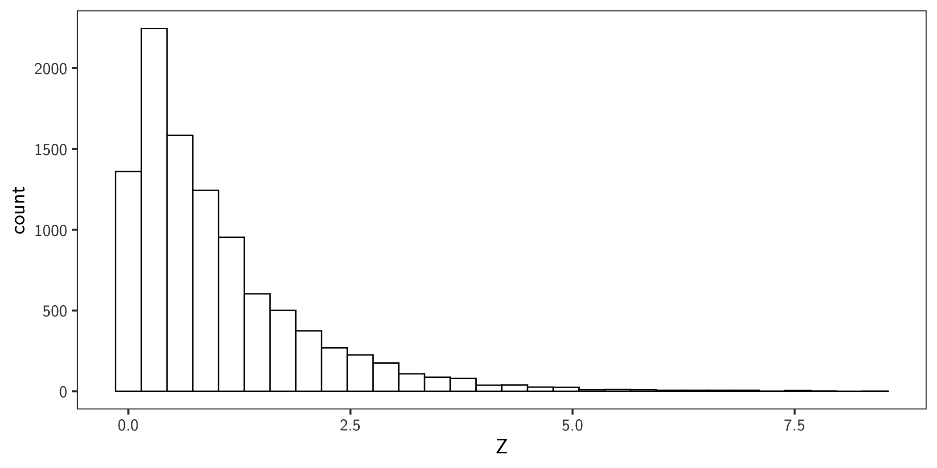
Let our desired random variable have the standard normal distribution.
Generating Random Variables
Benjamini-Hochberg False Discovery Rate (BH)
- Let FDR-BH be the expected value of FDP
\[\begin{align*} \text{FDR} &= \text{E}\left[Q\right] \\ &= \text{E}\left[\frac{V}{R} \Big| R > 0\right] \text{Pr}(R > 0) \end{align*}\]
- Let \(r_q\) be a value that controls the FDR at level \(q \in (0, 1)\) if
\[ \text{FDR}(r_q) < q \]
Benjamini-Hochberg False Discovery Rate (BH)
Decision rule:
- Consider an ordered set of \(p\)-values: \(\{p_i | i = 1, 2, ..., m\}\), where \(p_i \leq p_{i+1}\)
- Let \(r_q = \text{max}\{i: p_i \leq (i/m)q\}\)
- Then, let our rejection set be \(\{H_i\ \, | \, i \in (0, r_q)\}\)
Benjamini-Hochberg False Discovery Rate (BH)
Another method:
- Let \(k = \max\left\{i: p_i \leq \frac{i}{m}q\right\}\)
- Construct \(q_i^* = q(p_i) = \min_{i \leq k}\left(p_k \frac{m}{k}\right)\)
- Reject \(H_i\) if \(q_i^* \leq q\)
Bayesian FDR
- Let H be a binary random variable that takes the value 0 when a hypothesis is null, and 1 when a hypothesis is non-null
- Let \(m\) be the number of total hypotheses, \(m_0\) be the number of null, and \(m - m_0\) be the number of non-null
- \(\text{Pr}(H = 0) = \frac{m_0}{m} := \pi_0\)
- \(\text{Pr}(H = 1) = \frac{m - m_0}{m} = 1 - \pi_0 := \pi_1\)
- \(\pi_0\) is the a priori probability of null for each hypothesis
- In GWAS, \(\pi_0 >> \pi_1\)
- Assume that \(H \sim \text{Bernoulli}(\pi_i)\)
Bayesian FDR
- Our observed test statistics then have the marginal distribution
\[ p(z) = \text{Pr}(z | H = 0)\pi_0 + \text{Pr}(z | H = 1)\pi_1 \]
- Given a fixed rejection region \(A\), we denote its probability under the null or marginal marginal distributions as
\[ F_0(A) = \text{Pr}(Z \in A | H_0) = \int_A p_0(z)dz \]
\[ F(A) = \text{Pr}(Z \in A) = \int_A p(z)dz \]
Bayesian FDR
- Define the probability of a false discovery as
\[\begin{align*} \text{BFDR}(A) &= \text{Pr}(H = 0 | z \in A) \\[.5em] &= \frac{\text{Pr}(z \in A |H = 0) \text{Pr}(H = 0)}{\text{Pr}(Z \in A)} \\[.5em] &= \frac{F_0(A)\pi_0}{F(A)} \end{align*}\]
- Expected proportion of the false discoveries among all features considered significant
How to compute BFDR?
- Note that to compute BFDR, we require knowledge of
- \(\pi_0\), the a priori probability of a null hypothesis
- \(F_0\)
- \(F\)
- Empirical bayes approach: estimate these quantities from the data, and then approximate the BFDR
Empirical Bayes Estimation
- Consider that we have the results of a \(t\)-test for each of the \(m\) genes
- Assume \(F_0\) to be the standard normal distribution by transforming the \(p\)-values into \(z\)-values, set \(\pi_0\) to 1, and estimate \(F\) via:
\[\begin{align*} F(A) = \text{Pr}(Z \in A) &= \int_A p(z)dz \\ &= \int_{-\infty}^{\infty} I(z \in A)p(z)dz \\ &= \text{E}[I(z \in A)] \end{align*}\]
Which we empirically estimate via
\[ \hat{F}(A) = \hat{\text{Pr}}(Z \in A) = \frac{1}{m}\sum_{i=1}^m I(z_i \in A) \]
Empirical Bayes Estimation
Plugging that result in our empirical Bayes estimator, we achieve:
\[ \hat{BFDR}(A) = \frac{\hat{pi}_0 F_0(A)}{\hat{F}(A)} \]
- Posterior probability of false discoveries among the features whose \(z\)-values fall in the rejection region \(A\)
Using \(p\)-values as data
- If we set a threshold \(p_t\), where \(p_i \leq p_t \implies p_i \textsf{ is significant}\), we can then write
\[ F_0(p_t) = \text{Pr}(P_i \leq p_t \, |\, H_i = 0) = \int_0^{p_t} \text{Unif}(0, 1) = p_t \]
\[ F(p_t) = \text{Pr}(P \leq p_t) \]
\[ \hat{F}(p_t) = \hat{\text{Pr}}(P \leq p_t) = \frac{1}{m}\sum_{i=1}^m I(p_i \leq p_t) \]
and then estimate BFDR via
\[ \hat{BFDR}(p_t) = \frac{\hat{\pi}_0 p_t}{\frac{1}{m}\sum_{i=1}^m I(p_i \leq p_t)} \]
Example
snps <- 10000

# mixture of null and alternative p-values
p_values <- c(runif(snps * 0.9), runif(snps * 0.1, 0, 0.01))
p_t <- 0.05
significant <- p_values <= p_t
pi_0 <- seq(0, 1, length.out = 100)
bfdr <- (pi_0 * p_t) / mean(significant)

ggplot(data.frame(pi_0, bfdr), aes(x = pi_0, y = bfdr)) +
  geom_line() +
  labs(x = expression(pi[0]), y = "BFDR", title = "Bayesian False Discovery Rate")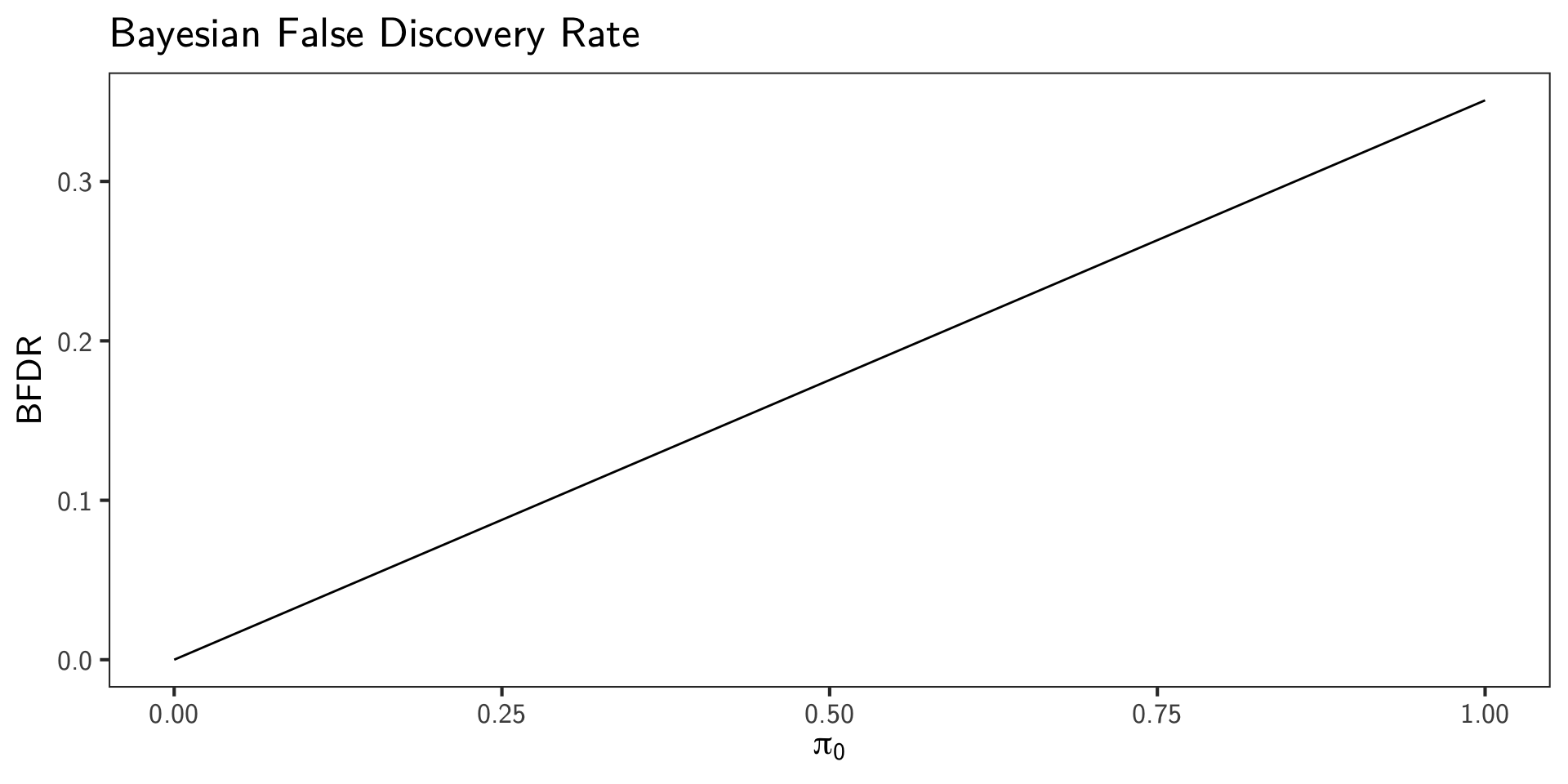
Local False Discovery Rates
- Note that FDR-BH and BFDR are interested in identifying a discovery set
- Instead, consider the probability of a false positive for a specific SNP \(j\) given that we observed \(y_j\):
\[\begin{align*} \text{fdr}(y_j) &= \text{Pr}(H_j = 0 \, | \, y_j) \\[.5em] &= \frac{p_0(y_j \, | \, H_j = 0) \pi_0}{p(y_j)} \qquad \textsf{(via Bayes' theorem)}\\[.5em] &= \frac{p_0(y_j \, | \, H_j = 0) \pi_0}{p_0(y_j \, | \, H_j = 0)\pi_0 + p_1(y_j \, | \, H_j = 1)(1 - \pi_0)} \end{align*}\]
- Given \(z\)-values, \(p_0 = \phi(y_j)\), \(\pi_0 := 1\)
- The denominator can be estimated using MLE or MCMC
\(q\)-values
- Formally,
\[ q(t) = \min_{\{A:t\in A\}}\left[pBFDR(A)\right] \]
- More intuitively, the \(q\)-value is the smallest pBFDR over all regions that reject \(H_i\)
- Expected proportion of false positives among all features as or more extreme than the one observed
- Empirical bayes estimate: \(q_i = q_i^* \hat{\pi}_0\)
- If the prior probability a randomly chosen hypothesis is null is 1, then the two values above are equal
\(q\)-values vs \(\alpha\)-values
- \(\alpha\)-value = \(\text{Pr}(\textsf{Test Positive} | H_0) =\) False positive rate
- \(q\)-value = \(\text{Pr}(H_0 | \textsf{Test Positive}) =\) False discovery rate
- \(q = .05 \implies\) “An estimated 5% of the results in the discovery set are false discoveries”
- \(\alpha = .05 \implies\) “An estimated 5% of all the tests performed are false discoveries”
Fully Bayesian FDR
We observe test statistics \(Z_1,\dots,Z_m\) (e.g., GWAS \(z\)‑scores) and introduce latent indicators \(H_i\in\{0,1\}\) with \[ H_i=0 \text{ (null)},\quad H_i=1 \text{ (non‑null)} \] \[ \Pr(H_i=0)=\pi_0,\ \Pr(H_i=1)=1-\pi_0. \]
Fully Bayesian FDR
Likelihood (symmetric, zero‑mean alternative):
\[\begin{align*} &Z_i \mid H_i=0 \sim \mathcal N(0,\tau^2) \\[.5em] &Z_i \mid H_i=1 \sim \mathcal N(0,\sigma^2) \end{align*}\]
(Allow \(\tau\neq 1\) to capture empirical‑null inflation/deflation.)
Fully Bayesian FDR
Priors (GWAS‑motivated):
\[\begin{align*} &\pi_0 \sim \mathrm{Beta}(20,1) \\ &\sigma \sim \mathrm{LogNormal}(0,0.5^2) \\ &\tau \sim \mathrm{LogNormal}(0,0.05^2) \end{align*}\]
Fully Bayesian FDR
Posterior over parameters \(\theta=(\pi_0,\sigma,\tau)\): \[ p(\theta\mid \mathbf z)\ \propto\ p(\theta)\ \prod_{i=1}^m\Big[\pi_0\,\phi_{\tau}(z_i) + (1-\pi_0)\,\phi_{\sigma}(z_i)\Big], \] with \(\phi_s\) the \(\mathcal N(0,s^2)\) pdf.
Fully Bayesian FDR
Local false discovery rate (per feature), integrating parameter uncertainty: \[ \operatorname{lfdr}_i =\Pr(H_i=0\mid z_i,\mathbf z) =\mathbb E_{\theta\mid\mathbf z}\!\left[ \frac{\pi_0\,\phi_{\tau}(z_i)} {\pi_0\,\phi_{\tau}(z_i)+(1-\pi_0)\,\phi_{\sigma}(z_i)} \right]. \]
Fully Bayesian FDR
Let a rejection rule be \(r_i(t)=\mathbf 1\{|z_i|\ge z_t\}\) where \(z_t=\Phi^{-1}(1-t/2)\). Define \[ R(t)=\sum_i r_i(t),\quad V(t)=\sum_i r_i(t)\,(1-H_i),\quad \mathrm{FDP}(t)=\frac{V(t)}{\max(1,R(t))}. \]
A fully Bayesian FDR at threshold \(t\) is the posterior expectation: \[ \boxed{\ \mathrm{FDR}(t)\ :=\ \mathbb E\!\left[\frac{V(t)}{\max(1,R(t))}\ \middle|\ \mathbf z\right] \ \approx\ \frac{1}{S}\sum_{s=1}^S \frac{\sum_i r_i(t)\,\operatorname{lfdr}_i^{(s)} }{\max(1,\sum_i r_i(t))}\ }, \] where \(\operatorname{lfdr}_i^{(s)}\) is the null posterior probability at draw \(\theta^{(s)}\).
Fully Bayesian FDR
Bayes‑optimal discovery set at level \(q\).
- Rank features by \(\widehat{\operatorname{lfdr}}_i=\mathbb E[\Pr(H_i=0\mid z_i,\theta)\mid \mathbf z]\)
- Let \(\bar\ell(k)\) be the running mean of the first \(k\) lfdrs.
- Choose \(\hat k=\max\{k:\bar\ell(k)\le q\}\) and take those \(\hat k\) features
- This minimizes posterior expected false discoveries among all sets of size \(\hat k\).
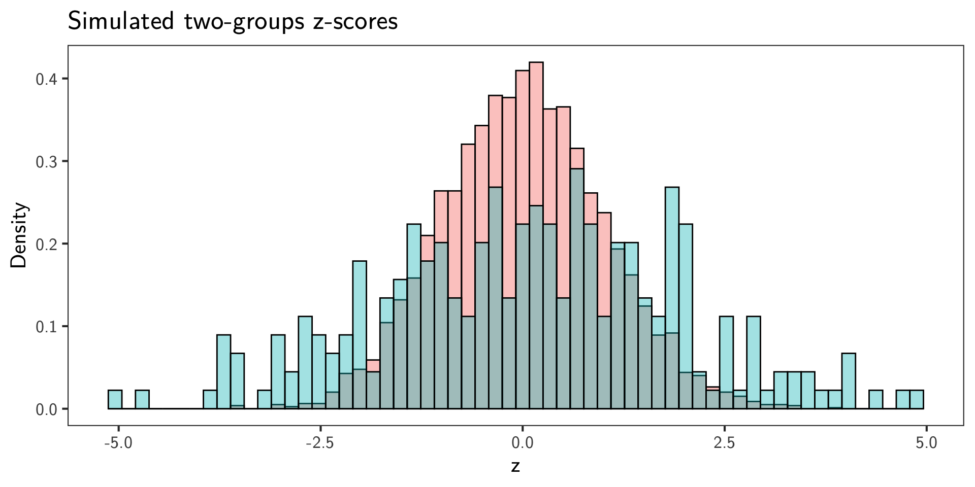
Simulate GWAS-like \(z\)-scores
- 1
- Choose parameters to control sparsity and scales.
- 2
- Encode the unknown truth via latent indicators in a two-groups model: \(H_i \sim \mathrm{Bernoulli}(1-\pi_0)\), so that on average \((1-\pi_0)m\) tests are non-null.
- 3
- Impose directional neutrality for two-sided testing by using a zero-centered alternative (no global shift of effects).
- 4
- Generate \(z\)-scores under the two-groups mixture. Null \(z\)-scores are centered at 0 with variance \(\tau^2\); non-null \(z\)-scores come from a zero-centered wider normal to induce heavy tails.
- 5
- Map \(z\)-scores to two-sided \(p\)-values under the standard normal null (\(\tau=1\)): \(p_i = 2\,\Phi(-|z_i|)\).
Simulate GWAS-like \(z\)-scores
Bayesian Two-Groups Fit (Stan)
- Model the marginal \(z\)-score density as a two-groups mixture:
\[ p(z_i \mid \theta) = \pi_0\, \varphi_{\tau}(z_i) + (1-\pi_0)\, \varphi_{\sigma}(z_i), \]
where \(\varphi_{\sigma}(\cdot)\) is the \(\mathcal N(0,\sigma^2)\) pdf. Priors encode GWAS sparsity and standard-null assumptions:
\[ \pi_0 \sim \mathrm{Beta}(20,1),\quad \sigma \sim \mathrm{LogNormal}(0,0.5),\quad \tau \sim \mathrm{LogNormal}(0,0.05). \]
- This matches the lecture: \(\pi_0 \gg \pi_1\) (sparse signals) and a tight null around 1 while allowing mild inflation.
Posterior Summary
| variable | mean | median | sd | mad | q5 | q95 |
|---|---|---|---|---|---|---|
| pi0 | 0.9299875 | 0.9345666 | 0.0313251 | 0.0280454 | 0.8676778 | 0.9703593 |
| sigma | 1.7883926 | 1.7657928 | 0.1873689 | 0.1780550 | 1.5202518 | 2.1319676 |
| tau | 0.9907577 | 0.9912889 | 0.0178861 | 0.0172593 | 0.9601886 | 1.0194893 |
- \(\pi_0\) is the estimated proportion of nulls
- \(\sigma\) is the estimated standard deviation of the alternative (zero-centered)
- \(\tau\) is the estimated standard deviation of the null
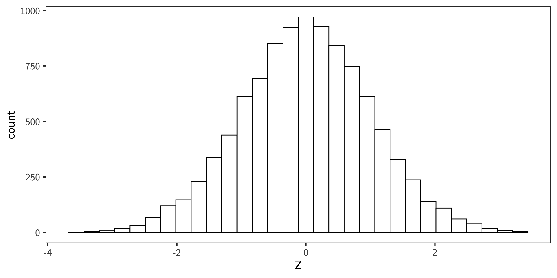
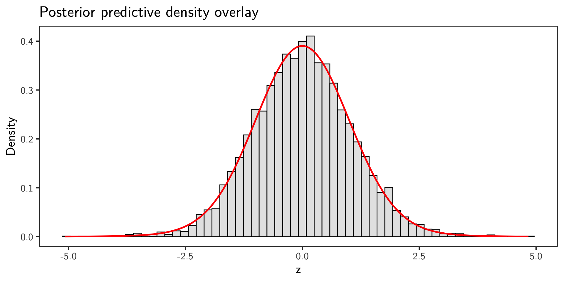
Posterior Predictive Check
- Posterior predictive density under parameters \(\theta=(\pi_0,\sigma,\tau)\) is
\[ p_\theta(z) = \pi_0\, \varphi_{\tau}(z) + (1-\pi_0)\, \varphi_{\sigma}(z). \]
- Overlay the posterior mean predictive density on the \(z\) histogram.
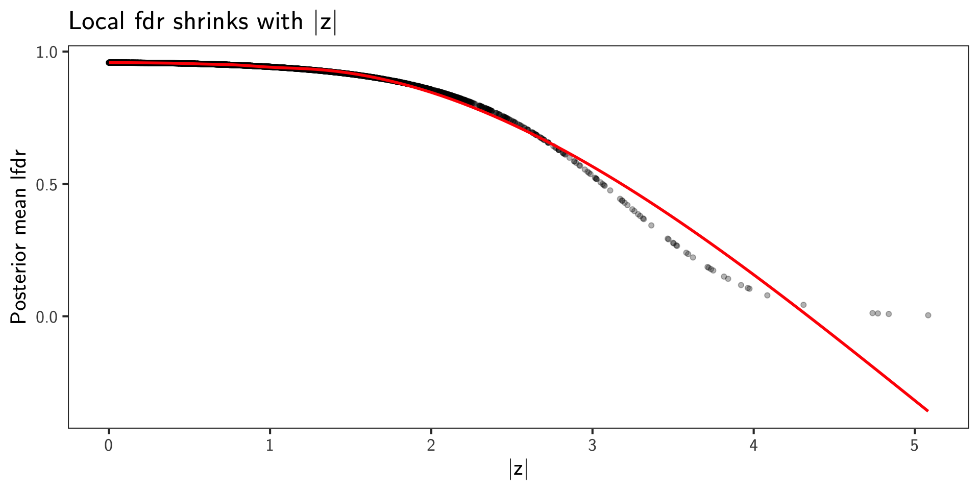
Posterior Local fdr
- The local false discovery rate for SNP \(i\) is the posterior probability of null given \(z_i\) and parameters:
\[ \operatorname{lfdr}_i(\theta) = \Pr(H_i=0 \mid z_i,\theta) = \frac{\pi_0\,\varphi_{\tau}(z_i)}{\pi_0\,\varphi_{\tau}(z_i) + (1-\pi_0)\,\varphi_{\sigma}(z_i)}. \]
Posterior Local fdr
- Our Stan model returns
lfdrin generated quantities. Compute posterior means \(\hat{\operatorname{lfdr}}_i\) and visualize.
`geom_smooth()` using method = 'gam' and formula = 'y ~ s(x, bs = "cs")'