library(glmnet)
set.seed(3337)
# X,y should be prepared beforehand
cv.out <- cv.glmnet(X, y, alpha=1, intercept=TRUE, family="binomial", type.measure="class")
bestlam <- cv.out$lambda.min
coef(cv.out, s=bestlam)
pred_class <- predict(cv.out, s=bestlam, newx=X, type="class")
pred_prob  <- predict(cv.out, s=bestlam, newx=X, type="response")
err_rate   <- mean((as.numeric(pred_class)-y)^2)
brier <- mean((as.numeric(pred_prob)-y)^2)Lecture 08: Binary Data
PUBH 8878, Statistical Genetics
Binary classification overview
Setup. Observations \((Y_i, x_i)\) with \(Y_i\in\{0,1\}\), \(x_i\in\mathbb{R}^p\).
- A classifier returns a score \(s(x_i)\in[0,1]\)
- We predict \(\hat Y_i=\mathbf 1\{s(x_i)>t\}\) for threshold \(t\in[0,1]\).
- With \(s(x)=\Pr(Y=1\mid x)\) and \(t=0.5\), Bayes rule minimizes \(\Pr(\hat Y\neq Y)\).
Two viewpoints.
- Direct probability (GLM): model \(\pi(x)=\Pr(Y=1\mid x)\) via a link \(g\); logistic uses \(g=\mathrm{logit}\), probit uses \(g=\Phi^{-1}\).
- Latent‑threshold (liability): let \(U=\mu+x^\top\beta+\varepsilon\) and \(Y=\mathbf 1\{U>0\}\). If \(\varepsilon\sim\mathcal N(0,1)\) we obtain probit; if \(\varepsilon\) is logistic we obtain logistic.
Types of models
Logistic model
\[ \Pr(Y=1\mid x)=\frac{\exp(x^\top\beta)}{1+\exp(x^\top\beta)},\quad \text{logit}\,\Pr(Y=1\mid x)=x^\top\beta . \]
Probit model
\[ \Pr(Y=1\mid x)=\Phi(\mu+x^\top b),\quad \Phi^{-1}\Pr(Y=1\mid x)=\mu+x^\top b . \]
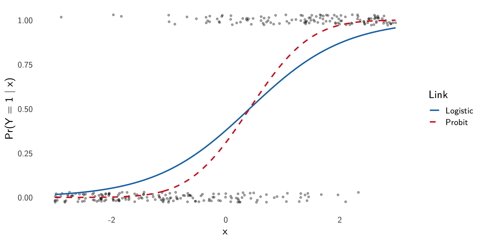
Logit vs probit: one predictor
Visual comparison. For a single covariate \(x\), fix \((\mu,\beta)\) and plot \[ \pi_{\text{logit}}(x)=\mathrm{logit}^{-1}(\mu+\beta x),\quad \pi_{\text{probit}}(x)=\Phi(\mu+\beta x),\quad \]
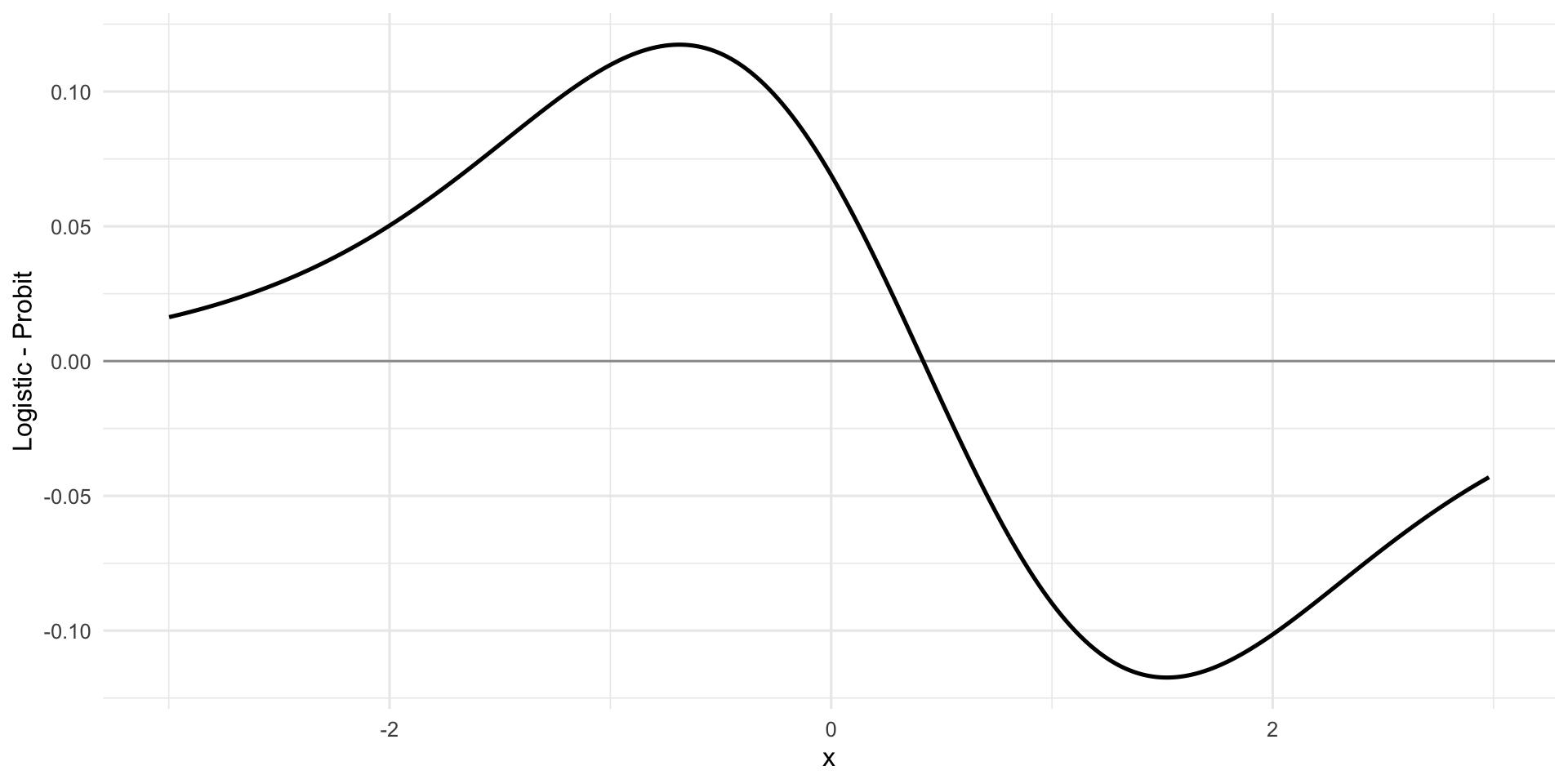
Logit vs probit: one predictor
Visual comparison. For a single covariate \(x\), fix \((\mu,\beta)\) and plot
\[ \Delta(x)=\pi_{\text{logit}}(x)-\pi_{\text{probit}}(x) \]
Losses for binary outcomes
0–1 error / error rate: \((y_i-\hat y_i)^2\) equals \(1\) if misclassified, \(0\) otherwise.
Training vs validating MSE:
\[ \widehat{E}(\mathrm{MSE}_v) =\frac{1}{N}\sum_{i=1}^N (y_i-\hat y_i)^2 + \frac{2}{N}\sum_{i=1}^N \mathrm{Cov}(\hat y_i,y_i) \] where the second term is expected optimism.- Why it appears. Because \(\hat y_i\) is fit using \(y_i\), they co‑move: training loss looks too small. On fresh data (independent of the fit), this advantage vanishes, so loss increases.
- Interpreting \(\mathrm{Cov}(\hat y_i,y_i)\). It measures how much the prediction at \(i\) chases noise in \(y_i\)
- more model flexibility increases this covariance (more optimism), while regularization/shrinkage reduces it.
Losses for binary outcomes
- Brier score (probability forecasts):
\[ \mathrm{MSE}^{\text{Brier}}_v=\frac{1}{N_v}\sum_{i=1}^{N_v}\big(y_i-\hat \pi_i\big)^2. \]
Penalized logistic regression (ridge)
We minimize \[ J(\mu,\beta)= -\ell(\mu,\beta\mid y,X)+\frac{\lambda}{2}\lVert \beta\rVert_2^2 \] \[ \ell=\sum_{i=1}^n\Big[y_i f_i-\log\{1+\exp(f_i)\}\Big] \]
\[ f_i=\mu+x_i^\top\beta \]
Logistic lasso
Solve \[ \max_{\beta_0,\beta}\;\sum_{i=1}^n \Big[ y_i(\beta_0+x_i^\top\beta)-\log\{1+\exp(\beta_0+x_i^\top\beta)\}\Big] -\lambda\sum_{j=1}^p|\beta_j|, \] with standardized predictors, unpenalized intercept.
Bayesian spike-and-slab (binary via probit)
Latent liability: \(U_i=\mu+x_i^\top b + e_i\), \(e_i\sim\mathcal N(0,1)\); \(Y_i=\mathbf 1\{U_i>0\}\).
Spike-slab prior: \(b_j=\alpha_j\delta_j\), \(\alpha_j\sim\mathcal N(0,\sigma_b^2)\), \(\delta_j\sim\mathrm{Bernoulli}(\pi)\).
Bayesian spike-and-slab
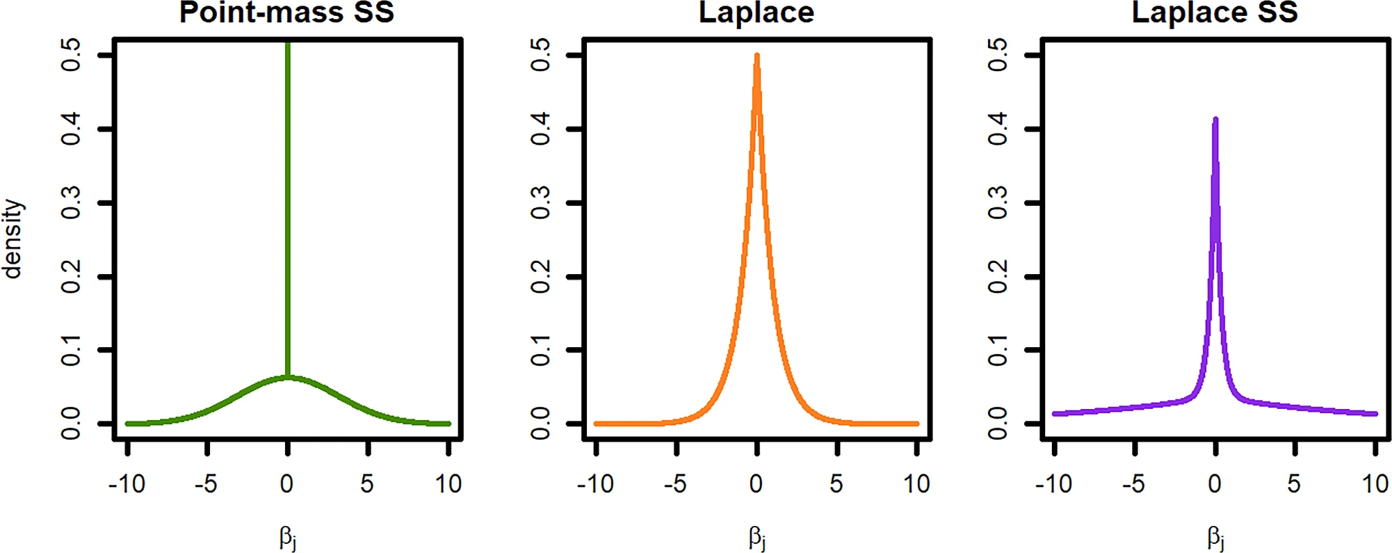
Biziaev et al. (2025)
ROC curves and AUC
- True Positive Rate (TPR): \(\text{Pr}(\hat{Y} = 1 | Y = 1)\)
- False Positive Rate (FPR): \(\text{Pr}(\hat{Y} = 1 | Y = 0)\)
- True Negative Rate (TNR): \(\text{Pr}(\hat{Y} = 0 | Y = 0)\)
- False Negative Rate (FNR): \(\text{Pr}(\hat{Y} = 0 | Y = 1)\)
- Prevalance or Incidence: \(\text{Pr}(Y = 1)\)
I will use these terms instead of sensitivity and specificity
ROC curves and AUC
- Receiver operating characteristic curve (ROC(t)): plot \(\mathrm{TPR}(t)=\Pr(s(X)>t\mid Y=1)\) against \(\mathrm{FPR}(t)=\Pr(s(X)>t\mid Y=0)\).
- Area under the curve (AUC): The area under the curve of the ROC is a measure of model performance
- AUC can be understood as the probability that a random positive is ranked higher than a random negative:
\[\begin{align*} \mathrm{AUC} &=\Pr\big(s_1>s_0\big) \\ &=\int_{-\infty}^{\infty}[1-F_1(t)] f_0(t)\,dt \\ &=\iint \mathbf 1\{u>t\} f_1(u) f_0(t)\,du\,dt \end{align*}\]
ROC curves and AUC
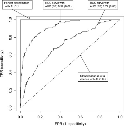
Parikh and Thiessen Philbrook (2017)
Choosing a threshold
- \(t=0.5\) minimizes the overall error rate \(\Pr(\hat Y\neq Y)\) when \(s(x)=\Pr(Y=1\mid x)\).
- But clinical priorities may prefer lower FNR at the expense of higher FPR.
Example: rare disease prevalance
- Prevalance of a disease is the proportion in the population that have the disease: \(\text{P}(\hat{Y} = 1)\)
- Given a random sample of \(n\) individuals, we generate predictions \(\hat{Y}\) using some rule \(s(x)\), which declares \(T\) individuals as positive, so
\[ \widehat{\text{Pr}}\left(\hat{Y} = 1\right) = \frac{T}{n} \]
Example: rare disease prevalance
- What’s the relationship between \(\text{P}(\hat{Y} = 1)\) and \(\text{P}(Y = 1)\)?
\[ \text{P}(\hat{Y} = 1) = \underbrace{\text{P}(\hat{Y} = 1 | Y = 1)}_{\text{TPR}}\text{P}(Y = 1) + \underbrace{\text{P}(\hat{Y} = 1 | Y = 0)}_{\text{FPR}}\text{P}(Y = 0) \]
- Thus, we instead compute the unbiased estimator:
\[\begin{align*} \frac { \text{P}(\hat{Y} = 1) - \text{P}(\hat{Y} = 1 | Y = 0) } { \text{P}(\hat{Y} = 1 | Y = 1) - \text{P}(\hat{Y} = 1 | Y = 0) } &= \frac{T - n(\text{P}(\hat{Y} = 1 | Y = 0))}{n(\text{P}(\hat{Y} = 1 | Y = 1) - \text{P}(\hat{Y} = 1 | Y = 0))} \\[1em] &= \frac{(T/n) - \text{FPR}}{\text{TPR} - \text{FPR}} \end{align*}\]
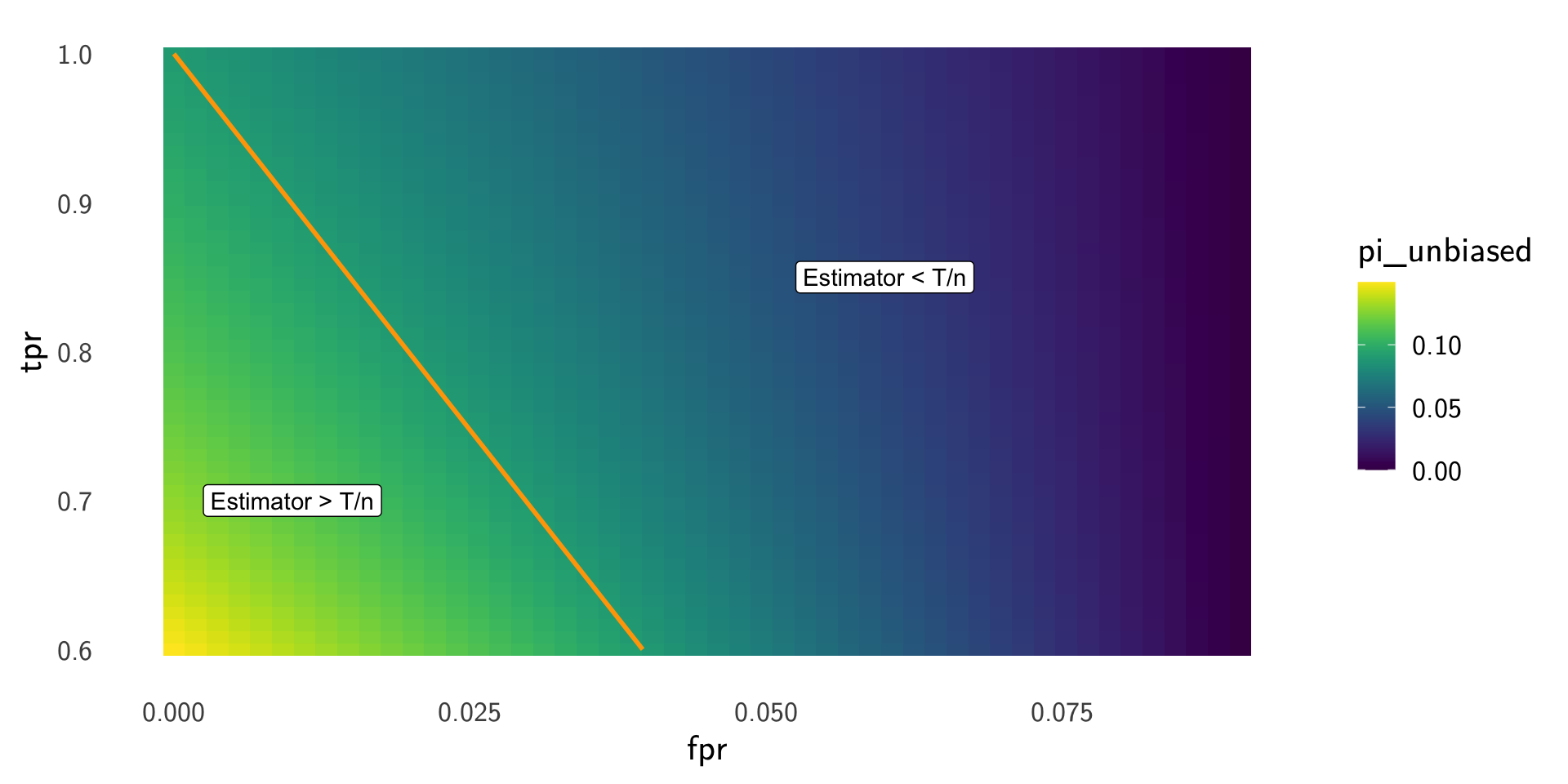
Example: rare disease prevalance
Fix the observed positive rate \(T/n\) and vary \((\mathrm{TPR},\mathrm{FPR})\) to see how the prevalence estimate \[ \widehat{\pi}=\frac{T/n-\mathrm{FPR}}{\mathrm{TPR}-\mathrm{FPR}} \] changes.
Example: rare disease prevalance
Example: rare disease prevalance
- This correction requires knowledge of the test’s operating characteristics.
- Use TPR, FPR, TNR, FNR terminology:
- TPR = Pr(\(\hat Y=1\mid Y=1\)), FNR = \(1-\text{TPR}\)
- FPR = Pr(\(\hat Y=1\mid Y=0\)), TNR = \(1-\text{FPR}\)
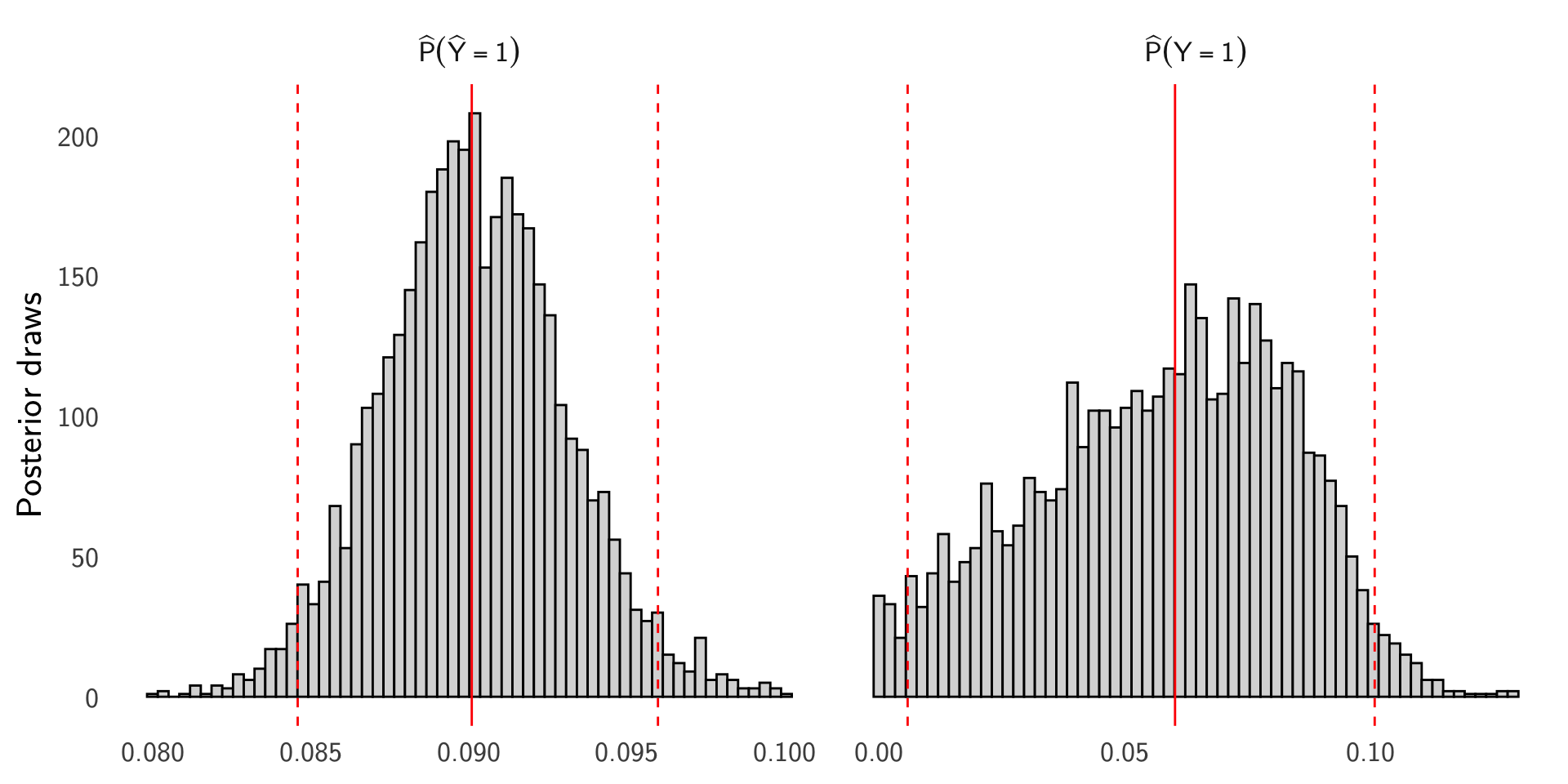
- We can use a Bayesian model to account for uncertainty in TPR and FPR and infer prevalence \(\pi\).
- Example. \(n=10{,}000\), \(T=900\), \(\text{TPR}\approx0.85\), \(\text{TNR}\approx0.95\) (so \(\text{FPR}\approx0.05\), \(\text{FNR}\approx0.15\)).
Bayesian model with cmdstanr. Let \(T\sim\mathrm{Binomial}\big(n,\,\pi\,\mathrm{TPR}+(1-\pi)\,\mathrm{FPR}\big)\) with Beta priors for \(\pi\), TPR, and FPR. Stan program saved at lectures/stan/prevalence_from_pred.stan.
Posterior histograms
Example: GWAS
Spike-Slab Model
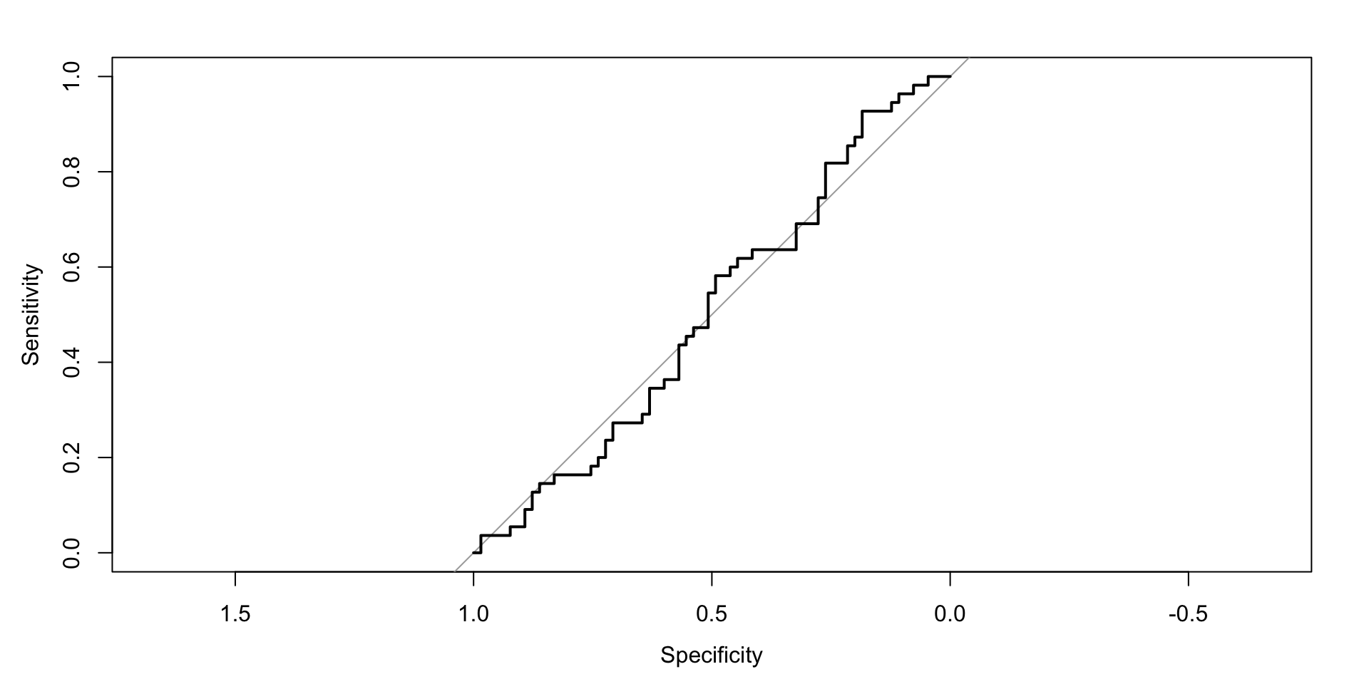
Consider a probit model for \(Y_i\in\{0,1\}\) with genotypes \(X_i\in\{0,1,2\}^p\): \[ \Pr(Y_i=1\mid X_i)=\Phi(\alpha+X_i^\top\beta) \]
Spike-and-slab prior on \(\beta_j\): \[ \beta_j=\alpha_j\delta_j,\quad \alpha_j\sim\mathcal N(0,\sigma_b^2),\quad \delta_j\sim\mathrm{Bernoulli}(\pi) \]
Goal: identify associated variants (nonzero \(\beta_j\)) and predict case/control status.
Spike-Slab Model ROC
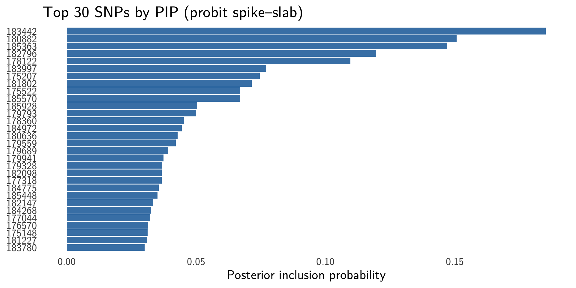
Spike-Slab Posterior Inclusion Probabilities (PIPs)
PIP is the posterior probability that SNP \(j\) is included in the model
Polygenic Risk Scores (PRS)
- A PRS is a weighted sum of genotype dosages, \(PRS_i = Σ_j x_{ij} w_j\), used to estimate an individual’s genetic liability or risk. It is a linear predictor like the ones we’ve fit, applied genome‑wide(Choi et al., 2020)
- From individual‑level data: learning \(w\) is exactly the supervised learning we covered
- Evaluation: report Brier/ROC‑AUC/PR‑AUC and calibration on held‑out data, assess across ancestry groups when relevant
Other Predictive Models and Scores
- Beyond linear PRS: random forests, gradient boosting, SVMs, neural nets, and deep learning can capture non‑linear effects and interactions
- Not always PRS‑compatible: these models produce complex functions of all SNPs, you cannot summarize them as a single vector of per‑SNP weights
- Many ML models output scores that are not well‑calibrated probabilities, post‑hoc calibration (e.g., Platt scaling, isotonic regression) may be needed for risk communication (Guo et al., 2017; Niculescu-Mizil and Caruana, 2005).
- Shareability/portability: PRS is easy to share (weights) and recompute, black‑box models typically require access to the full model object and identical feature preprocessing, and may transport poorly across ancestries (Duncan et al., 2019; Martin et al., 2019).
PRS from Summary Statistics
- Setup: summary statistics give, for each SNP j, a marginal effect \(\hat{\beta}_j\) (and SE, p‑value, sample size) from a GWAS; we do not have individual genotypes \(X\).
- Why LD matters: SNPs are correlated (linkage disequilibrium, LD). If you naively use \(\hat{\beta}_j\) as weights, nearby correlated SNPs can be counted multiple times. “Clumping+thresholding” (C+T) keeps one SNP per LD region to reduce double‑counting but discards signal (see Choi et al., 2020).
PRS from Summary Statistics
- LD matrices: let \(R = \operatorname{cor}(X)\) be the LD (correlation) matrix.
- In‑sample LD: correlations computed from the original GWAS training genotypes. With individual‑level data, your model implicitly uses this through \(X^{\top}X\).
- Reference LD: when only summary stats are available, we approximate LD using a separate reference panel (e.g., 1000G or a matched biobank subset) chosen to match the ancestry and QC of the target data.
- LD‑aware summary methods (big picture): jointly shrink correlated \(\hat{\beta}\) using the LD matrix \(R\) to get adjusted effects \(\hat{w}\) you can apply to target genotypes. Examples: LDpred/LDpred2 (Privé et al., 2020; Vilhjálmsson et al., 2015), PRS‑CS (Ge et al., 2019), lassosum (Mak et al., 2017).
PRS from Summary Statistics
Typical pipeline (summary‑level PRS):
- Harmonize alleles, build the intersecting SNP set across summary stats, LD reference, and target.
- Construct block‑wise LD matrices \(R_b\) from the reference (e.g., 1–3 cM windows).
- Provide z‑scores or \((\hat{\beta}, \mathrm{SE}, N)\) to the method along with \(R_b\).
- Run an LD‑aware algorithm (e.g., LDpred2‑grid/auto, PRS‑CS) to obtain posterior mean effects.
- Compute PRS in the target by \[\mathrm{PRS} = X_{\text{target}}\, \hat{w}\] and evaluate on held‑out data.
References
Biziaev, T., Kopciuk, K. and Chekouo, T. (2025) Using prior-data conflict to tune Bayesian regularized regression models. Stat Comput, 35, 1–19. Springer US. DOI: 10.1007/s11222-025-10582-1.
Choi, S. W., Mak, T. S.-H. and O’Reilly, P. F. (2020) Tutorial: A guide to performing polygenic risk score analyses. Nature Protocols, 15, 2759–2772. DOI: 10.1038/s41596-020-0353-1.
Duncan, L., Shen, H., Gelaye, B., et al. (2019) Analysis of polygenic risk score usage and performance in diverse human populations. Nature Communications, 10, 3328. DOI: 10.1038/s41467-019-11112-0.
Ge, T., Chen, C.-Y., Ni, Y., et al. (2019) Polygenic prediction via Bayesian regression and continuous shrinkage priors. Nature Communications, 10, 1776. DOI: 10.1038/s41467-019-09718-5.
Guo, C., Pleiss, G., Sun, Y., et al. (2017) On calibration of modern neural networks. In: Proceedings of the 34th international conference on machine learning, 2017, pp. 1321–1330.
Mak, T. S. H., Porsch, R. M., Choi, S. W., et al. (2017) Polygenic scores via penalized regression on summary statistics. PLOS Genetics, 13, e1007128. DOI: 10.1371/journal.pgen.1007128.
Martin, A. R., Kanai, M., Kamatani, Y., et al. (2019) Clinical use of current polygenic risk scores may exacerbate health disparities. Nature Genetics, 51, 584–591. DOI: 10.1038/s41588-019-0379-x.
Niculescu-Mizil, A. and Caruana, R. (2005) Predicting good probabilities with supervised learning. In: Proceedings of the 22nd international conference on machine learning, 2005, pp. 625–632. ACM. DOI: 10.1145/1102351.1102430.
Parikh, C. R. and Thiessen Philbrook, H. (2017) Chapter Two - Statistical Considerations in Analysis and Interpretation of Biomarker Studies. In Biomarkers of Kidney Disease (Second Edition) (ed. C. L. Edelstein), pp. 21–32. Academic Press. DOI: 10.1016/B978-0-12-803014-1.00002-9.
Privé, F., Arbel, J. and Vilhjálmsson, B. J. (2020) LDpred2: Better, faster, stronger. Bioinformatics, 36, 5424–5431. DOI: 10.1093/bioinformatics/btaa1029.
Vilhjálmsson, B. J., Yang, J., Finucane, H. K., et al. (2015) Modeling linkage disequilibrium increases accuracy of polygenic risk scores. American Journal of Human Genetics, 97, 576–592. DOI: 10.1016/j.ajhg.2015.09.001.